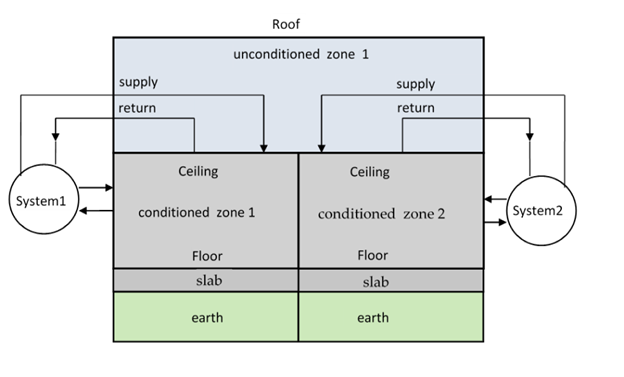
The building modeled can have multiple conditioned and unconditioned zones. Each conditioned zone has an air handler associated with it, and each air handler can have supply and/or return ducts in an unconditioned zone (nominally the attic), and in the conditioned zone itself. Air handlers can operate independently in either a heating, cooling, or off mode. See Figure 1.
Every time step (nominally two minutes), the zone model updates the heat transfers to and from the zones and the zone mass temperatures. Each zone’s conditions are updated in succession and independently, based on the conditions in the adjacent zones in the last time step.
The conditioned zone thermostat algorithms determine whether an air handler should be in a heating or cooling mode, or floating, and if heating or cooling, the magnitude of the load that must be met by the air handler to keep the conditioned zone at its current setpoint. If the setpoints cannot be satisfied, the conditioned zone floats with heating, cooling, or ventilation, at full capacity. In the off mode case the zones are modeled during the time step without duct or air handler effects.
Figure 1: Schematic of Zones and Air Handler Systems
Although shown partly outside of the envelope, all ducts are assumed to be in either the conditioned or unconditioned zones only.
The duct system model determines duct losses, their effect on the conditions of the unconditioned and conditioned zones, and their effect on the heating or cooling delivery of the air handler system.
The duct system model allows unequal return and supply duct areas, with optional insulation thicknesses. The ducts can have unequal supply and return leakages, and the influence of unbalanced duct leakage on the unconditioned and conditioned zones infiltration and ventilation is taken into account. Every time step it updates the air handler and duct system heat transfers, and HVAC energy inputs, outputs, and efficiency.
For each window, the ASHWAT window algorithm calculates the window instantaneous shortwave, longwave, and convective heat transfers to the zones.
The AIRNET infiltration and ventilation algorithm calculates the instantaneous air flow throughout the building based on the air temperatures in the zones, and on the outside wind and air temperature. AIRNET also handles fan induced flows.
In the update processes, a zones mass-node temperatures are updated using a forward-difference (Euler) finite difference solution, whereby the temperatures are updated using the driving conditions from the last time step. For accuracy, this forward-difference approach necessitates a small time-step.
The small time-step facilitates the no-iterations approach we have used to model many of the interactions between the zones, and allows the zones to be updated independently.
For example, when the zone energy balance is performed for the conditioned zone, if ventilation is called for, the ventilation capacity, which depends on the zone temperatures (as well as maximum possible ventilation openings and fan flows), is determined from the instantaneous balance done by AIRNET. To avoid iteration, the ventilation flows, and the accompanying heat transfers are based on the most recently available zone temperatures.
To avoid iteration, a similar use of the last time-step data is necessary is dealing with inter-zone wall heat transfer. For example, heat transfer through the ceiling depends on the conditions in both zones, but these conditions are not known simultaneously. Thus, ceiling masses are treated as belonging to the attic zone, and updated at the same time as other attic masses, partly based on the heat transfer from the conditioned zone to the ceiling from the last time step. In turn, when the conditioned zone is updated it determines the ceiling heat transfer based on the ceiling temperature determined two-minutes ago when the attic balance was done.
Similarly, when the conditioned zone energy balance is performed, if for example heating is called for, then the output capacity of the heating system needs to be known, which requires knowing the duct system efficiency. But the efficiency is only known after the air handler simulation is run. To avoid iteration between the conditioned zone and attic zones, the most recent duct efficiency is used to determine the capacity in the conditioned zones thermostat calculations. When the attic simulation is next performed, if the conditioned zone was last running at capacity, and if the efficiency now calculated turns out to be higher than was assumed by the thermostat calculations, then the load will have exceeded the limiting capacity by a small amount depending on the assumed vs. actual efficiency. In cases like this, to avoid iteration, the limiting capacity is allowed to exceed the actual limit by a small amount, so that the correct energy demand is determined for the conditioned zone load allowed.
Figure 2 shows a schematic of the zone model network. It models a single zone whose envelope consists of any number of walls, ceilings, floors, slabs, and windows, and can be adjacent to other conditioned or unconditioned zones. The envelope constructions can be made of any number of layers of different materials of arbitrary thermal conductivity and heat capacity. Each layer is modeled with one or more "T" networks in series. Each T has the layer heat capacitance, capij, centered between by two thermal conductances, where the first subscript corresponds to the wall construction number and the second to the layer number. Framed constructions are treated as two separate surface areas, the surface area of the part between framing, and the surface area of the part containing the framing itself; the heat flow is assumed to follow independent and parallel paths through these two surfaces.
Figure 2: Schematic of Simulation Network
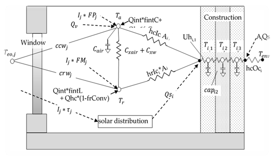
The room air,
represented by the mass node Ta, is assumed to be well-mixed and have heat
capacitance Cair (Btu/F). The air is shown in Figure 2 to interact
with all of the building interior construction surfaces via convection
coefficients hcIci for surface i. The overall conductance through the
window between
Ta and an effective outdoor temperature Teo is
ccwj for window surface j. The conductances ccwj
and the corresponding radiant value crwj are outputs of the ASHWAT
windows algorithm applied to window j each time step.
A mean radiant temperature node, Tr, acts as a clearinghouse for radiant exchange between surfaces. With conductances similar to those of the air node: hcIci and ccwj.
Depending on the size of the zone and the humidity of the air, the air is assumed to absorb a fraction of the long-wave radiation and is represented by the conductance CXair.
The internal gains, Qint, can be specified in the input as partly convective (fraction fintC ), partly long wave (fintLW), and partly shortwave (fintSW). The heating or cooling heat transfers are shown as Qhc (+ for heating, - for cooling). If Qhc is heating, a fraction (frConv) can be convective with the rest long-wave. The convective parts of Qint and Qhc are shown as added to the air node. The long wave fraction of Qint and Qhc are shown added to the Tr node.
Additional outputs of the ASHWAT algorithm are FPj the fraction of insolation Ij incident on window j that ultimately arrives at the air node via convection, and FMj, the fraction that arrives at the radiant node as long-wave radiation.
The term Qsi is the total solar radiation absorbed by each construction surface i, as determined by the solar distribution algorithm. The short wave part of the internal gains, Qint*fintSW, is distributed diffusely, with the same diffuse targeting as the diffusely distributed solar gains.
Solar gains absorbed at the outside surface of constructions are represented by Qso in Figure 2.
The slab is connected to the Ta and Tr in a similar fashion as the wall surfaces, although the slab/earth layering procedure is different than for walls.
Before a zone energy balance is formulated it is convenient to dissolve all the massless nodes from the network of Figure 2 (represented by the black dots), except for the mean radiant temperature node Tr. Figure 3 shows the resulting reduced network. A massless node is eliminated by first removing the short-wave gains from the node by using the current splitting principle (based on superposition), to put their equivalent gains directly onto adjacent mass nodes and other nodes that have fixed temperatures during a time step. Then the massless node can be dissolved by using Y-Δ transformations of the circuit.
Figure 3: Network after Dissolving Massless Nodes
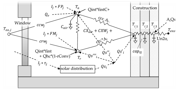
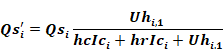
For example, to eliminate the massless surface node of layered mass in Figure 2, the gain Qsi absorbed by the surface node is split into three parts: Qsi' to the Ti, 1 node, Qsi'' to the Ta node and Qsi''' to the Tr node. For example, by current splitting, Qsi'
Equation 1
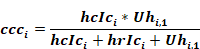
A Y-Δ transformation of the remaining Y circuit gives the ccci and crci conductances, as well as an additional cross conductance CXCi that is added to CXair. For example,
Equation 2
The temperatures in the zone are determined using a thermal balance method. The following procedure is followed each time step.
At the start of the simulation, say time t, assume all temps Ta(t),Tr(t),Ti,1(t),Ti,2(t), etc. are known along with all the solar gains, internal gains, etc.
(1) First, the layered mass temperatures are updated using the explicit Euler routine (see Section 2.2), giving Ti,1 (t+dt), Ti,2(t+dt), etc. The Euler method determines each of these mass temperatures assuming that all the boundary conditions (temperatures and heat sources) that cause the change in the mass temperatures, are conditions at time t. Thus the mass node temperatures can be in any order, independently of each other.
(2) Next, a steady-state instantaneous energy balance at the Ta and Tr nodes is made at time t+ dt. This balance involves the mass temperatures determined for time t + dt in Step-1, as well other heating or cooling sources at time t+ dt. The balance in this step involves querying the HVAC control algorithm which allows heating, cooling and ventilation (forced or natural) in response to scheduled setpoints. The idealized control system is assumed to keep the zone at exactly the scheduled setpoint unless Ta is in the deadband or if the HVAC capacity is exceeded, whereupon the system runs at maximum capacity, and Ta floats above or below the relevant setpoint. While the heating, cooling and forced ventilation system capacities are scheduled inputs, the natural ventilation capacity is dependent on the current zone and environment conditions.
Thus, the energy balance at the Ta and Tr nodes returns either the heating, the cooling or the ventilation required to meet the setpoint, or else returns the floating Ta that results at the capacity limits or when Ta is in the deadband.
At this stage the conditions have been predicted for the end of the time step, and steps 1 and 2 and repeated. The various boundary conditions and temperature or air flow sensitive coefficients can be recalculated as necessary each time step at the beginning of step (1), giving complete flexibility to handle temperature sensitive heat transfer and control changes at a time step level.
Note that step (2) treats the energy balance on Ta as a steady state balance, despite the fact that air mass makes it a transient problem. However, as shown in Section 2.3.1, if the air mass temperature is updated using an implicit-difference method, the effect of the air mass can be duplicated by employing a resistance, Δt/Cair, between the Ta node and a fictitious node set at the beginning of the time-step air temperature TaL = Ta(t), and shown as such in Figure 3.
The overall CSE Calculation Sequence is summarized below:
Hour
Determine and distribute internal gains.
Sub-hour
Determine solar gain on surfaces.
Determine surface heat transfer coefficients.
Update mass layer temperatures.
Find AirNet mass flows for non-venting situation (building leakage + last step HVAC air flows).
Find floating air temp in all zones / determine if vent possibly useful for any zone.
If vent useful
•find AirNet mass flows for full venting
•find largest vent fraction that does not sub-cool any zone; this fraction is then used for all zones.
•if largest vent fraction > 0, update all floating zone temperatures assuming that vent fraction
Determine HVAC requirements for all zones by comparing floating temp to setpoints (if any)
•System heating / cooling mode is determined by need of 1st zone that requires conditioning
•For each zone, system indicates state (t and w) of air that could be delivered at register (includes duct loss effects). Zone then requests air flow rate required to hold set-point temperature
Determine HVAC air flow to zones (may be less than requested); determine zone final zone air temperatures.
Determine system run fraction and thus fuel requirements.
Determine zone humidity ratio for each zone.
Calculate comfort metrics for each zone.