The radiation coefficients for surfaces inside the conditioned zone are given in Section 2.6.1 where the long-wave radiant network model is discussed.
The wind velocity as a function of height at the house site is obtained from the meteorological station wind measurement by making adjustments for terrain and height differences between the meteorological station and the house site.
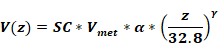
This method uses Equation 36 which determines the wind velocity V(z), in ft/sec, at any height z (ft) based on the wind velocity, Vmet in ft/sec, measured at a location with a Class II terrain (see Table 1) and at a height of 10-meters (32.8 ft):
Equation 36
where,
α and γ are obtained from Table 1 for the terrain class at the building location.
SC = shielding coefficient from Table 2 for the building location.
Vz=wind velocity at height z at the building location (ft/sec).
Vmet = wind velocity (ft/sec) measured at 10-meters height in a Class II location.
The terrain factor of Table 1 is a general factor describing the influence of the surroundings on a scale on the order of several miles. The shielding factor of Table 2 is a local factor describing the influence of the surroundings on a scale of a few hundred yards.
Table 1: Parameters for Standard Terrain Classifications
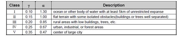
Table 2: Local Shielding Parameters
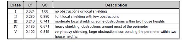
If it is assumed that the default value of the terrain classification at the building location is Class IV terrain of Table 1, and the default local shielding coefficient is SC= 0.571 of Class IV of Table 2, then the wind velocity at the building site at height z is given by:

or,
For example, for 1, 2, and 3 story buildings, of 9.8 ft (3-m), 19.7 ft (6-m), and 29.5 ft (9-m), respectively, then the local eave height wind velocities are:
V(9.8)
 met for a 1-story building.
V(19.7) = 0.34 Vmet for a 2-story building.
V(29.5) = 0.38 Vmet for a 3-story building.
(References: Sherman & Grimsrud (1980), Deru & Burns (2003), Burch & Casey (2009), European Convention for Constructional Steelwork (1978).)
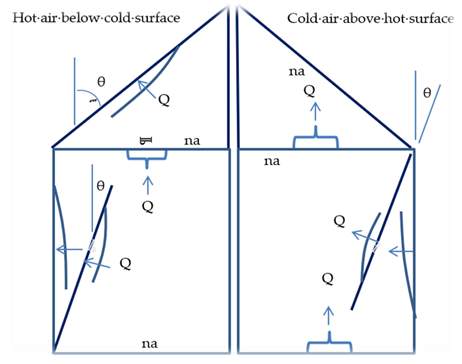
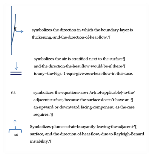
The schematic buildings in Figure 4 and Figure 5 show all of the possible interior heat transfer situations for which the convection heat transfer coefficients are determined. The figures symbolically show the nature of the heat transfer boundary layer, and the heat flow direction. The symbols used are explained at the end of this document. Similar schematics have not been done for the outside surfaces.
The equations are developed that give the heat transfer coefficient for each of the Figure 4 and Figure 5 situations, and for the building outside surfaces. The heat transfer coefficients depend on the surface tilt angle θ (0 ≤ θ ≤ 90), the surface and air temperatures, and on whether the heat flow of the surface has an upward or downward facing component.
The results, which apply to both the UZ and CZ zones, can be summarized as follows:
For floors, and either vertical walls, or walls pulled-in-at-the-bottom:
If Tair > Tsurf use Equation 53. (heat flow down)
If Tair < Tsurf use Equation 52. (heat flow up)
For ceilings (horiz or tilted), and walls pulled-in-at-the-top:
If Tair > Tsurf use Equation 52. (heat flow up)
If Tair < Tsurf use Equation 53. (heat flow down)
For all vertical walls, and walls with moderate tilts use Equation 54.
For horizontal or tilted roof, use Equation 57.
Figure 4: Heat Flow Down Situations
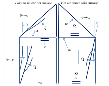
Figure 5: Heat Flow Up Situations
Explanation of Symbols
Equation 37, from Churchill and Chu (see Eq. 4.86, Mills (1992)), is used to determine the natural convection coefficients for tilted surfaces. The choice of this equation is partly informed by the work of Wallenten (2001), which compares the Churchill and Chu equation with other correlations and experimental data.
Equation 37 is for turbulent convection (109 <Ra <1012), expected to be the dominant case in room heat transfer.
Equation 37 applies to either side of a tilted surface for angles (0 ≤ θ ≤ 88o) if the heat flow has a downward component, or the heat flow is horizontal.
Equation 37 also applies to either side of a tilted surface for angles θ <600 of the heat flow has an upward component, or the heat flow is horizontal.
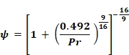
Equation 37

where,
Ra = the Rayleigh number.
Nu = the Nusselt number.
Pr = the Prandtl number.
Using
 Equation 37 reduces to:
Equation 38

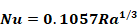
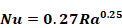
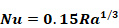
For high Ra [Ra≈>109] , neglecting the additive terms “1” and “0.68” in Equation 37 gives:
Equation 39
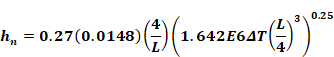
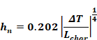
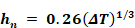
By the definition of the Nusselt number, the natural convection heat transfer coef, hn is:
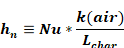
At 70F,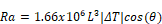
and k=0.0148, Equation 39 reduces to:
Equation 40
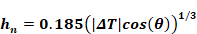
Note that hn is independent of characteristic length Lchar
Downward heat flow
According to Mill’s(1992) Equation 37 doesn’t apply to downward heat flow for .θ>88o At 70 F, for a 20 ft characteristic length, the 0.68 term predicted by Equation 38 for θ=90o corresponds to hn=0.68k/L=0.0005; essentially zero. Although the downward heat flow is ideally stably stratified (three cases shown in Figure), most measurements and modeling practice indicate h may be larger than zero. We use the equation of Clear et al. for the minimum, for heat flow down:
Equation 41
Clear’s equation reduces to:
Equation 42
or
where, Lchar is the wall characteristic length; see Equation 52 definitions.
Adding this h to Equation 40 gives:
Equation 43
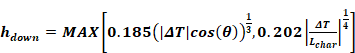

The following simplification is made, where the exponent of the second term is changed to 1/3, so that |ΔT|1/3 can be factored out:
Equation 44
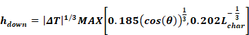
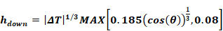
Changing the exponent means Equation 44 gives same answer as Equation 43 only when ΔT/Lchar =1. But Equation 44 would have acceptable error for other ΔT/Lchar ratios, and gives more or less the right dependence on ΔT. If in addition, one assumes a typical Lchar=15, say,then the minimum term becomes: 0.202L-1/3/char=0.08 , giving the final reasonable form:
Equation 45
Upward heat flow for 
For the inside & outside of walls where the heat flow has an upward (or horizontal heat flow at the limit θ=0o), and the outside of roofs, Equation 40 applies:
Upward heat flow for 
To handle cases of upward heat flow for θ>60o, hups is found by interpolating between, Equation 40 evaluated at θ=60o, and Equation 47 at 900 Equation 46 , for heat transfer from a horizontal surface (θ=90) is from Clear et al. (Eq. 11a). It is close to the much used McAdams equation suggested by both the Mills(1992) and Incropera-Dewitt textbooks.
Equation 46
At 70-F, Equation 46 reduces to
Equation 47
Interpolating, for upward heat flow cases with

which reduces to:
Equation 48
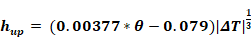

where θ is in degrees.
Measured forced convection heat transfer coefficients are frequently correlated using an equation of the form
Equation 49
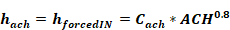
The RBH model (Barnaby et al. (2004) suggests using hf=0.88 Btu/hr-ft2F at ACH = 8. This gives Cach= 0.167. Walton (1983) assumes h = 1.08 when the “air handler system is moving air through the zone.” If this was at 8 ach, then this implies Cach=0.205.
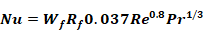
From Clear et al. (2001, Eq. (11a)),
Equation 50
Clear et al. used the Reynolds number based on a free-stream wind velocity 26.2 ft (8 m) above the ground.
At 70F, Equation 50 reduces to:
Equation 51
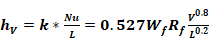
where for walls,


 wind velocity at eave height at
building
location, in ft/sec,
wind velocity at eave height at
building
location, in ft/sec, 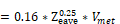 from Section 2.5.1.2.
 freestream wind velocity, in
ft/sec, 10 m (32.8 ft) above the ground at the meteorological station
site.
freestream wind velocity, in
ft/sec, 10 m (32.8 ft) above the ground at the meteorological station
site.
Rf=Table 3 value.

The wind direction multiplier, Wf, is defined as the average h of all of the vertical walls, divided by the h of the windward wall, with this ratio averaged over all wind directions. We estimated Wf using the CFD and wind tunnel data of Blocken et al. (2009) for a cubical house. Blocken’s Table 6 gives a windward surface convection coefficient of hc≈4.7V0.84 (SI units), averaged over wind direction. Blocken’s Figure 9 gives (hc )≈7.5
averaged over all vertical surfaces, for wind speed - Vmet=3m/s. Thus, we estimate . ----9u
and for roofs,
 roof
roof
 =
=

V = wind velocity 9.8 ft (3 m) above the eave height at
i00building location, in ft/sec.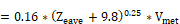

Rf = Table 3 value.
Walton (1983) assumed that the ASHRAE roughness factors of Table 3 apply to the convection coefficient correlations. The Clear et al. (2001) experiments tend to confirm the validity of these factors. Blocken et al. (2009) says, “The building facade has been assumed to be perfectly smooth. Earlier experimental studies have shown the importance of small-scale surface roughness on convective heat transfer. For example, Rowley et al. found that the forced convection coefficient for stucco was almost twice that for glass. Other studies showed the important influence of larger-scale surface roughness, such as the presence of mullions in glazed areas or architectural details on the facade, on the convection coefficient.”
Table
3: Surface Roughness Parameter
|
Roughness Index |
Rf |
Example |
|
1 (very rough) |
2.1 |
Stucco |
|
2 (rough) |
1.67 |
Brick |
|
3 (medium rough) |
1.52 |
Concrete |
|
4 (Medium smooth) |
1.13 |
Clear pine |
|
5 (Smooth) |
1.11 |
Smooth plaster |
|
6 (Very Smooth) |
1 |
Glass |
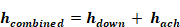
The combined convection coefficient is assumed to be the direct sum of the natural and forced convection coefficients:
For upward and horizontal heat flow:
Equation 52

where,
hup= Equation 40 or Equation 48 depending on whether θ is < or > 60o.
hach= Equation 49
For downward heat flow:
Equation 53
where,
hdown = Equation 45
hach = Equation 49
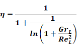
The conclusion of Clear et al. (2001) is that the combined convection coefficient is best correlated by assuming it to be the sum of the natural and forced coefficients. For roofs, Clear et al. (2001) assumes that the natural and forced convection are additive, but that natural convection is suppressed by the factor η given by Equation 56 when forced convection is large (η → 0 as the Reynolds number becomes large). We also assume this attenuation of the natural convection applies to the outside of the walls.
For all vertical walls, and walls with moderate tilts:
Equation 54
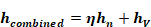
where,
hn = Equation 40
hv = Equation 51
(to avoid divide by zero, if V= 0, could set to V = 0.001)
where L & V are the same as used in Equation 51 for walls.
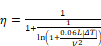
For roofs, Clear et al. (2001) assumes that the natural and
forced convection are additive, but that natural convection is suppressed by the
factor η → 0 as the Reynolds number becomes large). Clear gives η
as:
η → 0 as the Reynolds number becomes large). Clear gives η
as:
Equation 55
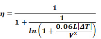
At 70F, with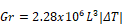 2, and L=Lchar for surface , Equation 55
reduces to:
2, and L=Lchar for surface , Equation 55
reduces to:
Equation 56
For roofs:
Equation 57
where,
hn = Equation 45 for downward heat flow.
hn = Equation 47 for upward heat flow.
hv =Equation 51 for upward or downward heat flow.
η is from Equation 56
L & V are the same as used in Equation 51 for roofs.
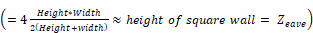
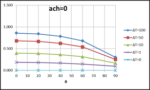
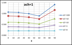
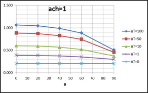
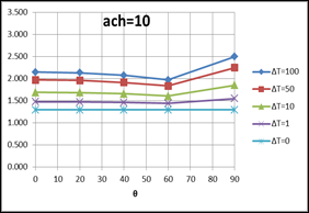
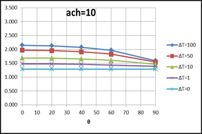
In Figure 6, the left hand column of plots are of Equation 53, for the downward heat flow cases shown in Figure 4. The right hand side plots are of Equation 52, for upward heat flow cases of Figure 5. All of the plots assume Tfilm=70F, and Lchar=Zeave=20 ft.
Figure 6: Plots of Equations for Downward and Upward Heat Flow
DOWNWARD HEAT FLOW (Equation 53): UPWARD HEAT FLOW (Equation 52):
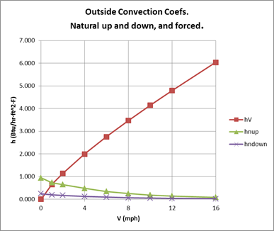
OUTSIDE surface convection coefficient Plot for a horizontal roof:
For


Figure 7: Outside Convection Coefficients, Natural Up and Down, and Forced
The net long wave radiation heat exchange between the outside surface and the environment is dependent on surface temperature, the spatial relationship between the surface and the surroundings, and the properties of the surface. The relevant material properties of the surface, emissivity ε and absorptivity α,are complex functions of temperature, angle, and wavelength. However, it is generally assumed in building energy calculations that the surface emits or reflects diffusely and is gray and opaque (α = ε, τ = 0, p = 1- ε)
The net radiant heat loss from a unit area of the outside of a construction surface to the outside environment is given by:
Equation 58

where,
ε = surface emissivity.
εg= ground emissivity is assumed to be 1.
α = Stephan-Boltzmann constant.
Ts = outside surface temperature.
Ta = outside dry bulb temperature.
Tg = ground surface temperature.
Tsky = effective temperature of sky.
Fgnd =view factor from surface to ground.
Fsky = view factor from surface to sky.

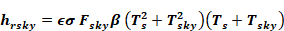
The sky irradiance is taken as a β weighted average of that from Tsky and that from Ta.
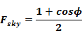
Howell (1982, #C-8, p.94), gives the fraction of the radiation leaving the window surface and reaching the sky by:
The fraction leaving the window incident on the ground is:
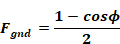
where, ϕ = surface tilt angle, the angle between ground upward normal and window outward normal (0o corresponds to a horizontal skylight, 90o to a vertical surface).
The parameter β accounts for the sky temperature’s approach to the air temp near the horizon. β is the fraction of the sky effectively at Tsky; (1-β) is the fraction of the sky effectively at Ta. β is used by Walton (1983), and Energy Plus (2009), but appears to have little theoretical or experimental basis.
Walton (1983) give β as:

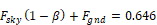
Since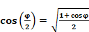 ,
,
it is noted that
Fsky=β2
and 
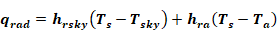
Equation 58 can be written as
Equation 59

where,

 is assumed to
be equal to Ta, so Equation 59 becomes
is assumed to
be equal to Ta, so Equation 59 becomes
Equation 60
where,
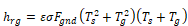
Equation 61
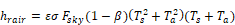
Equation 62

For a vertical surface,
so


Adding the exterior convection coefficient, hco, of Equation 40 to Equation 60 gives the total net heat transfer from the outside surface :
Equation 63

This can be written as,
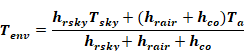
Equation 64
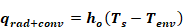
where ho is the effective exterior conductance to the conductance weighted average temperature, Tenv.
Equation 65
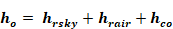
Equation 66
The ASHWAT window algorithm of Section 2.7 utilizes the irradiation intercepted by the window. From Equation 58 this can be deduced to be:
Equation 67
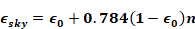
It is possible to approximate the long wave radiation
emission from the sky as a fraction of blackbody radiation corresponding to the
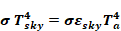
temperature of the air near the ground. The sky emittance εsky
is defined such that the sky irradiation on a horizontal surface is
The effective temperature of the sky is obtained by equating the blackbody emissive power of the sky at Tsky to the sky irradiation:
Equation 68
or,
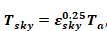
where Tsky and Ta are in degrees Rankine.
The value of  depends on
the dewpoint temperature, cloud cover, and cloud height data. Martin and Berdahl
(1984) give the εsky for clear skies as
depends on
the dewpoint temperature, cloud cover, and cloud height data. Martin and Berdahl
(1984) give the εsky for clear skies as
Equation 69

where,
 = the dewpoint temperature in
Celsius.
= the dewpoint temperature in
Celsius.
 = hour of day (1 to
24).
= hour of day (1 to
24).
 = atmospheric pressure in
millibars.
= atmospheric pressure in
millibars.
The clear sky emissivity is corrected to account for cloud cover by the following algorithm, developed by Larry Palmiter (with Berdahl’s imprimatur), that represents the Martin and Berdahl model when weather tape values of cloud ceiling height, and total and opaque cloud fractions are available.
Equation 70

where,
nop = the opaque cloud fraction
nth = the thin cloud
fraction:
n = the total sky cover fraction
εop = the opaque cloud emittance is assumed to be 1.
εth = the thin cloud emittance; assumed to be 0.4.
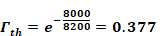
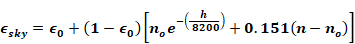
The cloud factor Γ is used to adjust the emissivity when the sky is cloudy due to the increasing cloud base temperature for decreasing cloud altitudes. The cloud base temperature is not available on the weather tapes, so assuming a standard lapse rate of 5.6oC/km, Γ is correlated with the more commonly measured cloud ceiling height, h (in meters), giving by the general expression:

For thin clouds, Γth is determined using an assumed cloud height of 8000-m, so,
Equation 71
For opaque clouds,
Equation 72

If ceiling height data is missing (coded 99999 on TMY2), the Palmiter model assumes that the opaque cloud base is at h=2000 m. If ceiling height is unlimited (coded as 77777) or cirroform (coded 88888), it is assumed that the opaque cloud base is at h=8000 m.
Using the assumed cloud cover and emissivity factors, Equation 70 becomes:
Equation 73

or,
In this case it is assumed that the cloud cover is opaque, ,
no=n when the ceiling height is less than 8000-m, and half opaque,
when the ceiling height is equal or greater than 8000. That is,
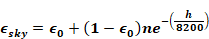
for h<8000 m (from Equation 73 with no=n):
Equation 74
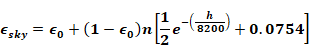
For (from
Equation 73 with
(from
Equation 73 with  ):
):
Equation 75
When only total sky cover is available using an h of 2000-m reduces Equation 74 to:
Equation 76