The CZM slab model is partly based on the Simplified Method for the calculation of heat flow through foundations, presented by Bazjanac et al. (2000). They divide a slab into two regions.
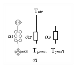
The perimeter area of the slab is defined as a 2 ft wide strip along external walls. Through this perimeter path, the interior air is assumed to be coupled via conductances α1, α2, and α3 to three environmental temperatures: ,Tweek ,Tground , and Tyear:
Figure 18: Perimeter Coupling
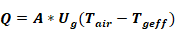
Thus the instantaneous heat flow from the room Temp node to perimeter slab, in Btu/hr-sf-F, is given by:
Equation 122

where,
Tair = the current interior-space effective temperature (involving both Ta and Tr).
Tweek = the average outside air temperature of the preceding two-weeks.
Tground = the current average temperature of the earth from the surface to a 10 ft depth.
Tyear = the average yearly dry bulb temperature.
α's = conductances from Table 3 of Bazjanac et al; Btu/sf-hr-F.
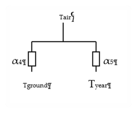
The core region couples T to Tground and Tyear, via conductances α4 and α5.
Figure 19: Core Coupling
Equation 123

Bazjanac et al. determined the conductances α1 through α5 by multi-linear regression analysis of the numerical results from a two-dimensional finite-difference slab-earth model. The conductances were determined for 52 slab foundation conditions and given in their Table 3.
The Bozjanac Table 3 conductances were obtained assuming the following properties:
1. Properties of earth:
conductivity = 1 Btuh/ft-F. (The k chosen was justified by assuming that lawns and other vegetation around California houses was watered during the dry season).
density =115 lbm/ft3
specific heat = 0.2 Btu/lbm-F
thermal diffusivity = 0.0435 ft2/hr.
2 Slab: "heavy construction grade concrete"
thickness = 4-inches
conductivity = 0.8
density = 144
specific heat = 0.139
3 Rrug = 2.08 hr-ft2-F/Btu (ASHRAE 2005HF, p.25.5 'carpet fibrous pad').
4 Rfilm = 0.77 Btu/hr-ft2F, the inside surface-to-room-temperature combined convective and radiative conductance.
The above model uses the ground temperature determined by Kusuda and Achenbach (1965). Using the classical semi-infinite medium conduction equations for periodic surface temperature variation (Carslaw and Jaeger), they found the average ground temperature from the surface to a depth of 10 ft to be given by:
Equation 124

where,
 = average
outdoor temperature over year; F.
= average
outdoor temperature over year; F.
 = highest
average monthly outdoor temperature for the year; F.
= highest
average monthly outdoor temperature for the year; F.
 = lowest
average monthly outdoor temperature for the year; F.
= lowest
average monthly outdoor temperature for the year; F.
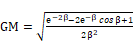 =
dimensionless amplitude for integrated depth average.
=
dimensionless amplitude for integrated depth average.
 =
dimensionless depth.
=
dimensionless depth.
L = 10 ft, the depth over which average is taken.
D = thermal diffusivity of soil, ft2/hr.
 hr = period
of 1 year.
hr = period
of 1 year.
Θ = 24(365M/12-15) ≈ elapsed time from Jan-1 to middle of month M; hours.
M = month, 1à12.
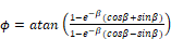 = phase angle for depth
averaged
= phase angle for depth
averaged  ; radians.
 radians =
phase lag of ground surface temperature (assumed equal to air temperature)
relative to January 1. From measured data, see Fig. 7 in Kusuda and
Achenbach.
radians =
phase lag of ground surface temperature (assumed equal to air temperature)
relative to January 1. From measured data, see Fig. 7 in Kusuda and
Achenbach.
The Bazjanac model assumes a constant indoor temperature, so cannot be applied directly to a whole building thermal-balance simulation model that allow changing indoor temperatures. To apply this model to CZM, with changing indoor temperatures, requires incorporating the dynamic effects of the slab and earth due to changing inside conditions.
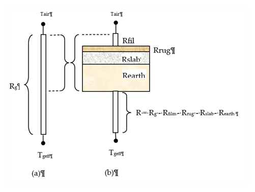
This is done by putting a one-dimensional layered construction, representing the slab and some amount of earth mass, into the steady-state Bazjanac model circuit--replacing part of its resistance by a thermal impedance (which is equal to the resistance for steady state conditions). In this way the correct internal temperature swing dynamics can be approximated.
First, the circuit of Figure 18 is alternately expressed as shown in Figure 20(a), with Equation 122 taking the form:
Equation 125
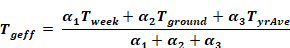
where Tgeff is the α-weighted average ground temperature:
Equation 126
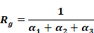
and
Equation 127
Similarly for the core region,
Equation 128
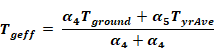
Equation 129

Now a one-dimensional layered construction is added into the circuit as shown in Figure 20(b), consisting of a surface film layer, a carpet (if any), the concrete slab, and earth layer. The bottom of the earth layer is then connected to Tgeff through the what's left of Rg.
A one-dimensional representation of the mass is appropriate for the core region. It is a bit of a stretch for the perimeter slab modeling, because the real perimeter heat flow is decidedly 2-dimensional, with the heat flow vectors evermore diverging along the path of heat flow.
Figure 20: Addition of Film, Rug, Slab, and Earth
The earth thicknesses required to adequately model the dynamic interaction between the room driving forces (sun and temperature) and the slab/earth model was determined by considering the frequency response of the slab earth model of Figure 20(b). In the frequency domain, the periodic heat flow from the Tair node is given by Equation 130.
Equation 130
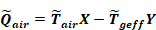
where,
X = the driving point admittance at the air (or combined air/radiant effective temp) node, in the units of Btu/hr-sf-F. It is the contribution to Q ̃air per degree amplitude of T ̃air X and Y are complex numbers determined from the layer properties (conductivity, heat capacity, density) of the circuit layers in Figure 20(b). See Carslaw and Jaeger; Subbarao and Anderson.
Y = the transfer admittance at the air node. It is the contribution to Q ̃air per degreee amplitude of .T ̃geff [The same value of transfer admittance applies to the Tgeff node, even if the circuit is not symmetrical, being the contribution to the T ̃geff node per degree amplitude of T ̃air]
Q ̃air = the amplitude (Btu/hr-ft2-F) and phase of the heat transfer rate leaving , T ̃air and is composed of the contribution from all of the frequencies that may be extant in the driving temperatures T ̃air and T ̃geff.
Note that the layers shown, when modeled as a mass construction, may need to be subdivided into thinner layers, particularly the earth, in order to satisfy the discretization procedure discussed in Section 2.4; but this subdivision is irrelevant to the slab model discussion in this section.
The maximum possible thickness of the earth layer is limited by the need for R to be positive. The limiting maximum possible thickness value, dmax, occurs in the perimeter case, when the foundation is uninsulated (i.e., the foundation insulation value R-0 in Bazjanac et al), and the slab is uncarpeted. In this case, dmax = 2.9 ft. The corresponding numbers for an uncarpeted core slab case is 11.8 ft
A depth of 2 ft is implemented in the code, for both the perimeter and core slab earth layers.
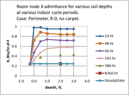
The 2 ft value was chosen primarily because, for the frequencies of concern, the magnitude of the X admittance from the Tair node was almost independent of earth layer depth for earth layer depths greater than 2 ft. See Figure 21. The phase shift is similarly essentially independent of depth after 2 ft. This was also the case for the core region.
This is the case for all indoor driving frequencies periods of up to at least 384-hr = 16-days. Thus 2 ft of earth is able to portray the dynamics resulting from a cycle of 8-cloudy days followed by 8 sunny days.
Figure 21: Room Node X Admittance
The transfer admittance Y shown in Figure 22 also contributes to Q ̃air according to the frequencies extant in the driving temperature .T ̃geff
Figure 22: Room Node Y Admittance
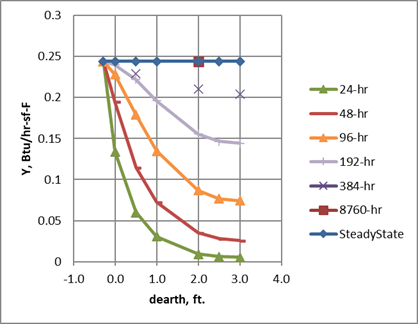
As seen in Equation 128, for the slab core region, T ̃geff has the same frequency content as Tground and Tyear. Tyear is a constant, i.e., zero frequency, steady-state.
As seen in Equation 124, Tground contains only the annual 8760-hr period. Figure 22 shows that the 8760-hr waves are transmitted unaffected by the mass layer. That is, Y becomes essentially equal to the steady state transfer admittance which is the U factor of the assembly, the reciprocal of the Rg value. Thus, for the core region, the magnitude of the slab loss rates produced by Equation 125 are preserved and unaffected by the added earth layers.
However, although the mass layers don't affect the magnitude of the Bazjanac model slab losses, they do introduce a time lag that is in addition to that already implicit in the T ̃geff values. For a 2 ft earth layer the lag is ~40-hours. A 22-day lag is already included by φ of Equation 124. To eliminate double-counting, the 40-hrs could be subtracted from phi, but this has not been done since 40-hr is inconsequential compared to 22 days.
For the perimeter region, T ̃geff has the the additional frequency content of the, Tweek the two-week running average outdoor temperature Tweek is dominated by the annual period, but has small amplitude 6-month period component, and a bit of signal at higher frequencies. Like the annual cycle, the 6-month period component is transmitted through the layered construction without damping, but again with a small but inconsequential phase lag.
Thus it was concluded that 2 ft of earth thicknesses below a 4-inch concrete slab adequately models changes in room side conditions, and at the same time adequately preserves the same average "deep earth" slab losses and phase lags of the Bazjanac model.
The validity of the response of the core slab construction is expected to be better than for the perimeter slab construction since the perimeter layers added do not properly account for the perimeter two-dimensional effects.
The longest pre-run warm-up time is expected to be for a carpeted core slab with the 2 ft earth layer. Using the classical unsteady heat flow charts for convectively heated or cooled slabs (Mills) , the time to warm the slab construction 90% (of its final energy change) was found to be about 20-days. Most of the heat-up heat transfer is via the low resistance rug and air film, with less through the higher ground resistance (R in Figure 20(b)), so the 20- day estimate is fairly valid for the complete range of foundation insulation options given in Bazjanac's Table 3.
Strictly speaking, the same properties assumed in the Bazjanac model in Section 2.8.1.3 should also be used in describing the rug, the concrete slab, and the earth in the layered constructions inputs.
This is particularly true for the carpet, if a carpet is specified, because the regression coefficients (the conductances a1, a2...) obtained for the carpeted slabs were sensitive to the Rrug value used. While inputting a different value than Rrug = 2.08 may give the desired carpeted room admittance response, the heat conducted from the deep ground will still give the heat flow based on Rrug = 2.08.
Small differences between the inputted and above properties is less important for the other layers, and is violated in the code with regard to Rfilm; its value is calculated each time-step and is used instead of 0.77, even though 0.77 is still the value subtracted from Rg in the code. This allows the correct modeling of the admittance of the slab floor, at the expense of a slight error in the overall resistance of the slab earth circuit.