This section describes the flow network algorithm used to model infiltration and ventilation air flows between conditioned zones, unconditioned zones, and the outdoors based on pressure and density differences and leakage areas between the zones.
Figure 23 shows the flow network interconnecting two conditioned zones (Z1 and Z2), the unconditioned attic and crawl space zones (Z3 and Z4), and the outside zone (Z5).
Figure 23. Schematic of Flow Network
The black lines represent one or more pressure difference driven and/or buoyancy driven flows between zones.
The blue lines in Figure 23 represent scheduled fan flows not directly dependent on zone-to-zone pressure differences. These include individual house fans (circled x's) and fan driven duct system supply, return, and leakages flows. The fans will affect the zone pressures, but the pressures won't affect the fan flow. The duct flows, determined by the load and air handler capacity, are assumed to not constitute leakage paths when the air handler is not operating.
Small leakage or ventilation openings will be modeled as orifices using a power law equations of Section 2.9.3 with an exponent of 0.5. Infiltration leaks are modeled with the power law equation exponent of 0.65.
Large vertical holes or infiltration surfaces, large enough that the vertical pressure difference distribution allows two-way flow, are modeled as two vertically separated small holes using the Wolozyn method (see Section 2.9.5 – Large Vertical Openings).
The following kind of elements are modeled using the power law equations:
•Wall infiltration for vertical envelope walls, vertical interzone walls, and roof decks
•Ceiling, floor, and wall base infiltration
•Interzone doors, door undercuts, jump ducts, relief vents
•Openable window flow
•Attic soffit vents, gable vents, roof deck vents, ridge vents
•Crawl space vents
•Trickle Vents
•Fire Place leakage.
•Infiltration to garage.
Additional equations are used to model large horizontal openings, like stairwells; Section 2.9.4. This type of opening would typically be between zones Z1 and Z2 in Figure 23 when the zones are stacked vertically. The algorithm used is based on that implemented in Energy Plus (2009). In addition to using the power law equation above, the algorithm calculates buoyancy induced flows that can occur when the density of the air above the opening is larger than the density of the air below the opening, causing Rayleigh-Taylor instability.
To determine the flow rates at each time step, the flow through each flow element in the building is determined for an assumed set of zone reference pressures. If the flow into each zones does not match the flow out of the zone, the pressures are adjusted by the Newton-Raphson iterative method until the flows balance in all the zones within specified tolerances.
For energy standards application, the air network for the four zone building model is designed to give results that are wind direction independent. In computing ventilation or infiltration air flows from holes in vertical walls exposed to outdoors, the program automatically calculates the sum of the flows through 4 holes each ¼ the area, one with each cardinal compass orientation, or an offset thereof. Thus, there will be wind induced flows through the envelope leakages that approximate the average flow expected over long periods, and they will be independent of wind direction. This approach is applied to all zone ventilation or infiltration flow elements connected to the outdoor conditions.
The pressure at a given elevation in a zone, including outdoors, is a combination of stack and wind effects added to the zones reference pressure. The difference in pressure in the zones on each side of a leakage element connecting the zones determines the flow rate through the element.
The pressure on the zone i side of a flow element is given by:
Equation 131
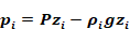
zi is the height of the element above some datum z=0. The datum is arbitrary but is nominally taken as ground level. Pzi is zone i's reference pressure. This is the pressure zone i would have at elevation z=0, regardless of whether the zone actually extends to this level. For the interior zones the Pzi reference pressures are the unknowns that are solved for using the Newton-Raphson method. This method determines what values of zone pressures simultaneously result in a balanced flow in each zone. The value of Pzi for the outdoor side of a flow element is given by (i is 5 if there are 4 conditioned and unconditioned zones):
Equation 132
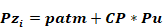
The weather tape atmospheric pressure, patm, is assumed to exist at the elevation z = 0 far from the building. Patm is taken as zero so that the unknown zones pressures will be found relative to the weather tape atmospheric pressure. Of course the actual weather tape atmospheric pressure is used in determining inside and outside zone air densities.
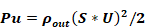
The wind velocity pressures, Pu, is:
Equation 133
where,
U is the wind velocity at eave height.
S is the shelter coefficient equal to SC of Table 2: Local Shielding Parameters.
ρout is the outside air density.
CP is the orientation sensitive pressure coefficient.
The wall pressure coefficients in Table 6 are those used by Walker et al. (2005). They are for the four vertical walls of an isolated rectangular house, with the wind perpendicular to the long wall (short wall = ½ long wall). As discussed in regard to hip roofs below, only data for the normal wind direction is used. These coefficients are used for all ventilation and infiltration holes in the walls. Soffit vents also use these values since they are assumed to have the same pressure coefficient as the walls under them. This assumption is roughly corroborated by the data of Sharples (1997).
Table 6: Pressure Coefficients for Wind Normal to One Wall
|
Wind Pressure Coefficient, CP | ||
|
Upwind wall |
Side walls |
Downwind Wall |
|
+0.6 |
-0.65 |
-0.3 |
Table 7 gives hip roof’s pressure coefficients for a range of roof angles. These are used to determine the outside pressure on ridge vents and roof deck vents.
There is little data available for hip roof surface pressure coefficients, or for ridge pressure coefficients (needed to model ridge vents) for any roof type. The data in Table 7 is a simplified synthesis of the data given by Xu (1998) and Holmes (1993, 2003, etc.), informed by a review of ASHRAE, EU AIVC, and other data sets and research papers.
Xu used a wind tunnel to measure pressure coefficients for a hip roofed building which was otherwise identical to the gable roof building wind tunnel data obtained by Holmes. The building had an aspect ratio of 2:1, with 0o wind direction normal to the long side (and normal to the gable ridge and hip roof top ridge). The building eave height was 0.4 the length of the short side. The building had a relatively large eave overhang of about 35% of the eave height. Xu and Holmes presented data for this building for roof pitch angles of 15, 20, and 30o . Other Holmes data, for both larger and smaller roof angles was used to estimate the pressure coefficients beyond the 15 to 30 degree range. Neither Xu nor Holmes presented average surface pressures, so the average surface data and average ridge pressures given in the table are based on estimates from their surface pressure contour data.
The table is for wind normal to the long side of the building. Similar tables were obtained from Xu's data for the 45 and 90 degree wind angles Table 7 would ideally be wind direction independent, implying some kind of average pressure coefficient; for example, for each surface take the pressure coefficient that is the average for the 0, 45, and 90 degree angles. However, infiltration flows depend on pressure differences, and the average of the pressure differences is not necessarily indicative of the difference of the average pressures. The soffit vents flows, driven by the pressure difference between the adjacent wall and the various roof vents complicate any averaging schemes.
Comparison of the pressure coefficients for the three wind
directions, while showing plausible differences, arguably does not show a
discernable pattern that would obviate just using the normal wind direction
data. Given the variety of roofs and building shapes that will be represented by
these coefficients, the variety of vent locations and areas, and the
deficiencies of the data, using a consistent set of data for only one wind
direction is deemed appropriate.
Table 7: Hip Roof Wind Pressure Coefficients
|
Roof Pitch |
Hip Roof Wind Pressure Coefficient, CP | |||
|
Upwind roof |
Side hip roofs |
Downwind Roof |
Ridge | |
|
|
-0.8 |
-0.5 |
-0.3 |
-0.5 |
|
|
-0.5 |
-0.5 |
-0.5 |
-0.8 |
|
|
-0.3 |
-0.5 |
-0.5 |
-0.5 |
|
|
+0.1(pos) |
-0.5 |
-0.5 |
-0.3 |
|
|
+0.3 (pos) |
-0.5 |
-0.5 |
-0.2 |
Zone i's air density ρi is assumed to be only a
function of zone temperature Ti That is, assuming the air is
an ideal gas, at standard atmospheric conditions, the pressure change required
to change the density by the same amount as a change in temperature of
1oF is  /
/  , which is
approximately - 200 Pascals/F. Since zone pressure changes are much smaller than
200 Pa, they are in the range of producing the same effect as only a fraction of
a degree F change in zone temperature; thus the density is assumed to always be
based on patm. (This has been changed in code so that ρi depends on both
Ti and Pzi).
, which is
approximately - 200 Pascals/F. Since zone pressure changes are much smaller than
200 Pa, they are in the range of producing the same effect as only a fraction of
a degree F change in zone temperature; thus the density is assumed to always be
based on patm. (This has been changed in code so that ρi depends on both
Ti and Pzi).
Using the ideal gas approximation, with absolute temperature units,
Equation 134

The pressure difference across the flow element is given by
Equation 135
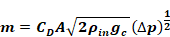
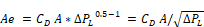
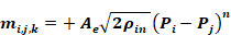
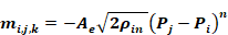
For an orifice, with fixed density of air along the flow path (from inlet to vena contracta), Bernoulli's equation gives:
Equation 136
where
CD is the dimensionless orifice contraction coefficient.
CD= π/(π+2) = Kirchoff’s irrotational flow value for a sharp edge orifice.
CD = 0.6 default for CSE windows
CD = 1 for rounded inlet orifice as used in ELA definition, and consistent with no vena contracta due to rounded inlet.
A = Orifice throat area, ft2.
ρin=
density of air entering the orifice;
The following is based on Sherman (1998). English units are used herein. Measured blower door infiltration data is expressed empirically as a power law:
Equation 137

Or
Equation 138

where
Q = volume flow in ft3/sec.
m = mass flow in
ρin= entering air density,
ΔP = pressure difference in
n = measured exponent, assumed to be n = 0.65 if measured value is unavailable.
κ = measured proportionality constant.
Equation 137 and Equation 138 are dimensional equations. Thus κ is not a dimensionless number but implicitly has the dimensions ft3+2n/(sec*lbfn). See Section 2.9.3.8–Converting Units of κ.
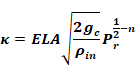
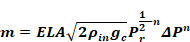
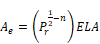
Sherman defines equivalent leakage area, ELA, as the
area of a rounded-entrance orifice that gives the same flow as the infiltration
of Equation 137 when the pressure difference ΔP is equal to
the reference pressure

 ΔP=Pr has a flow rate:
Equation 139
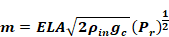
Equation 137 and Equation 139 with ΔP=Pr gives the ELA as:
Equation 140
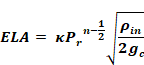
Solving Equation 140 for k, gives
Equation 141
Substituting Equation 140 into Equation 137 gives the general
equation, equivalent to Equation 137, that is the infiltration flow at any
pressure difference
Equation 142
(Note that substituting Equation 140 into Equation 142 recovers the empirical Equation 137).
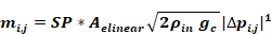
CSE uses Equation 136 to model flow through elements such as windows, doors, and vents. Equation 142 is used for infiltration flows for elements with a defined ELA.
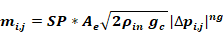
Both equations are special cases of the generalized flow power law Equation 143. For flow from zone i to zone j.
Equation 143
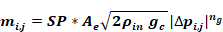
SP is the sign of the pressure difference ∆p(i,j)=pi-pj, utilized to determine the sign of the flow, defined as + from i to j . The exponent is ng “g” for generalized.
Equation 143 reduces to the orifice Equation 136 if:
•

•
Equation 143 reduces to the infiltration Equation 142 if:
•
where n here is the measured exponent.
•
•
[Although CD
is dimensionless in Equation 136 , the generalization to Equation 143 requires
CD to implicitly have the units of ].
].

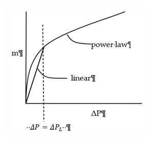
The partial derivative of the mass flow of Equation 143 with
respect to the pressure in zone
Equation 144
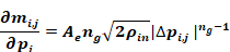
Since ng<1 this derivative à∞ asà zero, potentially causing problems with the
Newton-Raphson convergence. In order to make the derivative finite for small
pressure drops, whenever the pressure difference is below a fixed value, ∆PLthe
power law is extended to the origin by a linear power law
(ng=1),
Equation 145
as shown in Figure 24.
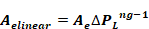
So that the flow rates match when ΔP=ΔPL,
Aelinear is determined by equating Equation 145 to Equation 143
with
Equation 146
Note that the derivative of m will be discontinuous when ∆p=∆PL, which conceivably could also cause Newton-Raphson problems, but during extensive code testing, none have occurred.
Figure 24: Mass Flow m versus Pressure Drop ΔP
The generalized flow equation, Equation 143,
is used with the following parameter values, depending on
element type and pressure drop
If
•
•A = area of flow element;
•
•
If
•
•A = area of flow element;
•
•
•∆PL = determined by computational experiment.
If
• , n
here is the measured exponent, or 0.65 if not known. (Note that if ,n =
0.65 Ae=1.45*ELA, used in CEC ACM manual).
•
•
•
o the measured parameters
 .
.
o code regulations, in which
case
If
•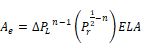
where n here is the measured value, or
•
The κ in Equation 137 is not dimensionless, so κ
changes value depending on the units of Q
and ΔP in Equation 137. The analysis herein
(Section 2.9) assumes Q in ΔP in
ΔP in
However, conventionally κ is obtained from measured data with ΔP in
Pascals. With these units Equation 137 takes the form:
ΔP in
Pascals. With these units Equation 137 takes the form:
Equation 147
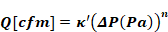
Using dimensional analysis the value of κ to be used in Equation 137 with Qin ft3/sec and ΔP in

Equation 148
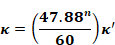
where the numbers are from the conversion factors
and 60 sec/min. κ=0.206 κ'for n = 0.65.
 the measured value from data with
  and
and  .
.
Using Equation 142 (in volume flow form) the infiltration volume flow, CFS50, with 50 Pa pressurization is:
Equation 149
CFS50 = ELA
where
ΔP = 50 Pa = 1.04428 psf
CFS50 = flow in units of
For cfm units, and ELA in square inches,
Equation 150
CFM50 = (60/144)CFS50 = 18.224*ELA
or alternately,
Equation 151
ELA [in2] = 0.055*CFM50
This is the equation used to get ELA from blower door data at 50 Pa pressure difference.
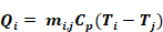
When the flow mi,j is positive, the heat delivered to zone j by this flow is given by
Equation 152
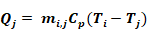
while the heat delivered to zone i by the flow mi,j is zero:
Equation 153

When the flow mi,j is negative, the heat delivered to zone j is zero,
Equation 154

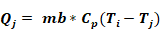
while the heat delivered to zone i by the flow mi,j is:
Equation 155
An additional set of equations is needed to model large horizontal openings such as stairwells. The algorithm used is similar to that implemented in Energy Plus, which is based on that given by Cooper (1989). In addition to pressure driven flow using the power law equations of Section 2.9.3.3 this algorithm involves buoyancy induced flows that can occur when the density of the air above the opening is larger than the density of the air below the opening, causing Rayleigh-Taylor instability.
For a given rectangular opening this algorithm can produce three separate flows components between the zones:
a) a forced orifice flow in the direction dictated by the zone to zone pressure difference, Δp. This flow is independent of the following instability induced flows.
b) a buoyancy flow downward when the air density in the upper zone is greater than that is the lower zone, i.e., Tupper-zone < Tlower-zone. This flow is maximum when Δp is zero, and linearly decreases with increasing Δp until the buoyancy flow is zero, which occurs when the pressure difference is large enough that the forced flow "overpowers" the instability flow. The latter occurs if Δp is greater than the "flooding" pressure ΔpF.
c) an upward buoyancy flow equal to the downward buoyancy flow.
These three flows are modeled by two flow-elements. The first element handles the forced flow (a) and in addition whichever of the buoyancy flow component, (a) or (c), that is in the same direction as the forced flow. The second element handles the alternate buoyancy flow component.
The pressure forced flow is modeled as orifice flow using Equation 143, except the area A in the Section 2.9.3.5 is replaced by:
Equation 156

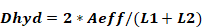
L1 and L2 are the dimensions of the horizontal rectangular hole. To include the effect of stairs, a StairAngle can be set, where StairAngle=90 deg corresponds to vertical stairs. The angle can be set to 90 degrees to exclude the effect of the stairs.
Equation 144 is used for the partial derivative of the flow,
with the area Ae using Aeff in place
of
When the zone on top has a higher density than the zone on the bottom, the maximum possible buoyancy flow, mbm, occurs when the pressure difference across the hole is zero:
Equation 157
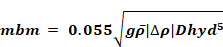
The 0.055 factor is dimensionless ; g = 32.2 ft/s2.
The hydraulic diameter of the hole is defined as:
Equation 158
When the zone on top has a higher density than the zone on the bottom, and the pressure difference is lower than the flooding pressure, then the buoyancy flow is given by:
Equation 159
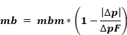
The flooding pressure difference ∆pF is defined as:
Equation 160
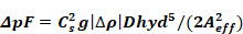
The shape factor
Equation 161
If the top zone density is lower than the bottom zones, or
if |∆p|>∆pF then the buoyancy flow mb is zero.
The partial derivatives of the buoyancy flows with respect to adjacent zone pressures are all zero since the buoyancy flows are equal and opposite. That is, although the buoyancy flow magnitudes are sensitive to zone pressures, they have no influence on the zone mass balance.
Although the buoyancy flows don't directly influence zone pressures, they do affect the heat transfer rates.
When buoyancy flows exists, the heat transfer due to the buoyancy flow to the upper zone, i say, is
Equation 162
and to the lower zone is
Equation 163
The flow through large vertical rectangular openings are handled using the method suggested by Woloszyn (1999).
Woloszyn uses a simplified version of the common integrate-over-pressure-distribution scheme as used by Walker for example. Rectangular holes are divided in two, with the flow through the top half driven by a constant Δp equal to the pressure difference ¾ the way up the opening (the midpoint of the top half of the opening area). Similarly, the flow through the bottom half uses the Δp at ¼ the way up the hole, and assumes it is constant over the bottom half. Although approximate compared to the integration methods, it is expected to be able to reasonably accurately, if not precisely, portray one and two way flows through such elements. This procedure has the virtue of eliminating the calculation of the neutral level, thereby greatly reducing the number of code logic branches and equations. It also eliminates a divide by zero problem when Δρ à 0 in the exact integration methods.
Besides being used for large vertical holes, like open windows and doorways, the method is also used for distributed infiltration. That is, a rectangular wall with an effective leakage area ELA is represented by two holes, each of area ELA/2, located at the ¼ and ¾ heights. These holes are then modeled using Equation 138, Equation 141, Equation 144, and Equation 145.
The method is generalized further to treat the tilted triangular surfaces assumed for hip roofs. In this case the lower Woloszyn hole, of area ELA/2, is placed at the height that is above ¼ of the area of the triangle. This can be shown to be a height of:
Equation 164
Similarly, the top hole is placed at the height above ¾ of the area of the triangle:
Equation 165
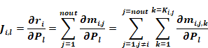
Assume there are a total of nuc conditioned and unconditioned zones with unknown pressures. The outside conditions, of known pressure, are assigned a zone number nout = nuc+1.
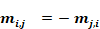
The mass flow rate from zone i to zone j (including j=nout) is designated as mi,j and can be positive (flow out of zone i) or negative (flow into zone i).
Equation 166
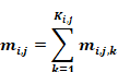
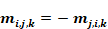
where mi,j,k is the flow rate through the k'th element of the Ki,j elements in surface i,j. By symmetry,
Equation 167
And
Equation 168
From Equation 167, mi,j,k values are functions of the zone pressure difference (Pi-Pj).
Equation 169

This shows that in general,
Equation 170
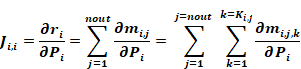
The net flow leaving zone i (i=1 to nuc) is the defined as the residual ri:
Equation 171
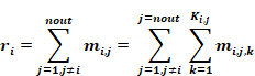
The j≠I criterion on the sums eliminates summing mi,i terms which are zero by definition. The zone pressures Pi are to be determined such that the residuals ri all become zero.
Equation 169 and Equation 171 constitute a set of n = nuc nonlinear equations with n = nuc unknown pressures. To linearize the equations, a Taylor's series is used to determine the residual ri 'at the pressure Pj' near the guessed value of pressures Pj, where the residual is ri Keeping only first order terms:
Equation 172
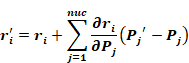
In matrix form this is written:
Equation 173
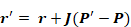
where r' is the vector with elements ri', and r is the vector with elements ri.
 is the nuc
by nuc Jocobian matrix with elements:
is the nuc
by nuc Jocobian matrix with elements:
Equation 174
where
Setting ri'=0 and solving for , Equation 173 becomes
Equation 175

Equation 176

where C is the correction vector:
Equation 177

Equation 178

Equation 178 gives the pressures Pj' that are predicted to make ri zero.
Convergence is attained when the residuals ri are sufficiently small. As employed by Energy Plus and Clarke, both absolute and relative magnitude tests are made.
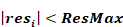
Convergence is assumed when the absolute magnitude of the residual in each zone i is less than a predetermined limit ResMax:
Equation 179
OR, the magnitude of the residual divided by the sum of the
magnitudes of the flow through each element connected to zone i, is less
than a predetermined limit
Equation 180
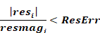
Where
Equation 181
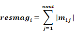
(code uses: sum of magnitude of flows to & from zone iz, resmag(iz) += ABS(mdot(iz,jz,ke)).
Equation 178 is more generally written as
Equation 182
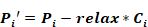
where relax is the relaxation coefficient, a factor less than one that reduces the correction applied to Pi. Relaxation factors on the order of 0.75 have been shown to reduce the number of iterations in cases normally having slowly decreasing and oscillating corrections. But a fixed value of 0.75 can slow what were formerly rapidly converging cases. The following approach is used to reduce the relaxation factor only when necessary.
Following Clarke, when the corrections Ci from one iteration to the next
changes sign, and the
latest Ci has a magnitude over half as big as the former
Ci, then it is assumed that the convergence is probably slow
and oscillating. This symptom is typically consistent over a few iterations, and
if this were precisely the case, the correction history would follow a geometric
progression with a negative common ratio 
Thus by extrapolation a better estimate of correct solution will be obtained if the relaxation factor is taken as the sum of the infinite termed geometric progression:
Equation 183
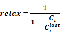
Thus, whenever, during an iteration for zone i,
Equation 184

then Equation 178 is replaced by
Equation 185
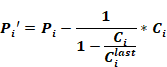
Insofar as the extrapolation is warranted, this should give a
better prediction of the pressure than would
using relax = 1 for this iteration. For the iteration following that
using Equation 185, relax = 1 is reverted to (i.e., Equation
178) so that only unrelaxed correction values are used to evaluate
than would
using relax = 1 for this iteration. For the iteration following that
using Equation 185, relax = 1 is reverted to (i.e., Equation
178) so that only unrelaxed correction values are used to evaluate
The following iteration, if any, is then again tested by
Equation 184. The first iteration is always done with relax = 0.75 since
at this point there is no value available for
It would be reasonable to add a max Ci limit; i.e., max pressure change allowed, a la Clarke, but code testing has not shown the need.
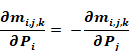
Consider Equation 174 for off-diagonal terms. Since i≠l, zone i's flow mi,j varies with Pl only if j = l. Thus setting lj = l,and i≠, Equation 174 reduces to:
Equation 186
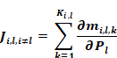
where
Equation 186, along with Equation 170, shows that all off
diagonal terms have a negative magnitude. Since
Equation 187
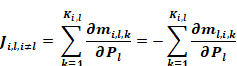
Using Equation 170, Equation 187 becomes:
Equation 188
Thus the Jacobian matrix is symmetric:
Equation 189

Thus only the upper (or lower) diagonal terms need be determined, with the other half determined by transposition. The off diagonal terms only involve partials of flows between zones with unknown pressures.
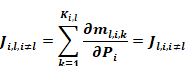
For i = j Equation 174 gives:
Equation 190
where
Equation 190 terms can be regrouped to show a simpler numerical way to determine Ji,i, by using the off diagonal terms already calculated:
Equation 191
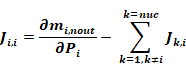
This shows that the diagonal elements use the derivatives of mass flows to the outdoors minus the off diagonal terms in the same column of the Jacobian.
Equation 191 shows that matrix will be singular
if 
so that at least one connection to outdoors is necessary.