The following algorithms are not currently implemented in the code, but are here for future code use, and in the interim are useful to manually determine the effects of screens on window ventilation flow pressure drop.
The references cited are a few of the papers reviewed to ascertain state of the art regarding screen pressure drop. In one of the more recent papers, Bailey et al. (2003) give the pressure drop through a screen as:
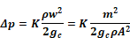
Equation B-1
where,
Equation B-2
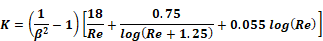
and,
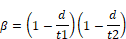
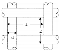
β = screen porosity = open area/total area perpendicular to flow direction.
 = Renolds number.
w = face velocity =
m = mass flow rate, lbm/sec.
d = wire diameter, ft.
ν = viscosity ≈ 1.25E-4 + 5.54E-07T(degF); ft2/sec. = 1/6100 ft2/sec at 70-F.
ρ = air density, lbm/ft3.
gc = 32.2 lbmft/lbf-sec2.
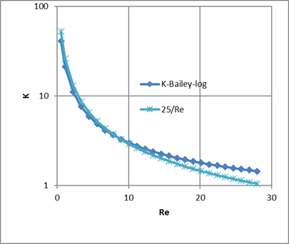
The first term, intended for portraying Re < 1 pressure drops, is the dominate term. The third term, intended for Re > 200, is relatively negligible, and the second term is a bridge between the first and third terms.
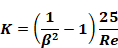
The Reynolds number for the screen flow
is roughly 5 times the face velocity in ft/sec. For a velocity of 1 ft/sec, Re ~ 5. For the expected range of wind speeds of concern for ventilation (see note #1), and with the motive of making the partial derivatives simple (see below), Equation B-2 is approximated as
Equation B-3
[note #1: California CZ12 ave yearly Vmet ≈ 11 ft/sec. Correcting for height and shielding gives Vlocal ≈ 11*0.5*0.32 ≈ 1.8 ft/sec. For max flow case of windows on windward and leeward walls, with typical wall wind pressure coefficients, w ≈ 0.5*Vlocal. Thus, the maximum window velocity expected for the annual average wind velocity of 11 ft/sec is w ≈ 0.5*1.8 = 0.9 ft/sec. In a building with windows in multiple directions, the average w is expected to be much lower, perhaps 0.5 ft/sec. Stack Effect: Using old ASHRAE equation, w(fpm)=9√(H[ft](ΔT[F]) = 9*√(10*10)/60=1.5 ft/sec. Together, the wind and stack may be on the order of 1-ft/sec].
The constant 25 in this approximate formula was determined by
forcing Equation B-2 and Equation B-3 to match when the window air velocity
is at the characteristic value
defined below. As discussed there, at this velocity the pressure drop through the screen is equal to that through the window orifice.
Figure B-1: Screen Pressure Drop
Equation B-3 can be written as
Equation B-4
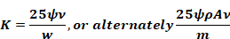
where, as a result of the approximation Equation B-3, the screen inputs can be combined into one characteristic screen parameter Ψ (of dimension ft-1 ):
Equation B-5
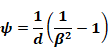
Ψ encapsulates all that needs to be known about the screen for pressure drop purposes. This is only true when K varies in the form assumed by Equation B-3.
The flow rate through a screenless window is modeled by Airnet as a sharp edged orifice of opening area A.
Equation B-6
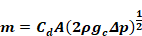
[Idelchik says this is valid for Re > 10^4].
At the equal pressure point the window orifice Reynolds
number is
wc = 1.89 ft/sec for std 14x18x0.011 screen &Cd=0.6; 14&18 are wires/inch.
Rec = 10.6 for std 14x18x0.011 screen &Cd=0.6
Rewdw= (~1.5*12/0.011)*(10.6)=1,7345 >104.
Thus Re is not > 104 when w < ~1 ft/sec. But this is when the pressure drop starts to be dominated by the screen, so the orifice drop accuracy is not so important.
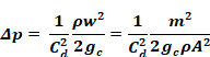
Solving for
Equation B-7
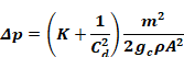
Adding Equation B-2 and Equation B-7 gives the total pressure drop for a window and screen in series:
Equation B-8
Solving for mass flow rate,
Equation B-9
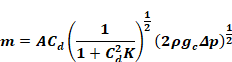
or,
Equation B-10
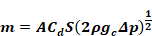
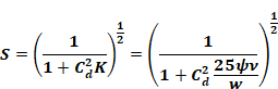
where S is the ratio of the flow with a screen to the flow rate without a screen, as a function of velocity w, viscosity, and screen and window orifice parameters.
Equation B-11
Equating Equation B-1 and Equation B-7 shows that the velocity when the screen and window pressure drops are equal is given by:
Equation B-12

The corresponding Reynolds number is
Substituting Equation B-12 into Equation B-11 shows that for this condition,
Equation B- 13
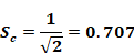
Equation B-12 and Equation B-13 show that ,wc which, besides viscosity, only depends on the screen constant Ψ and window-orifice coefficient Cd, can be considered a "characteristic" velocity, the velocity at which the flow is reduced by (1 - 0.707) ~ 29.3% by the addition of a screen to the window.
Figure B-2 shows that the typical Δp vs. flow curves for a screen and an orifice separately, not in series. The curves cross at velocity wc . To the left of wc, the laminar flow pressure drop dominates the window orifice pressure drop; to the right the orifice pressure drop progressively dominates. Screens give a greater flow reduction at low wind speeds than at high wind speeds.
Figure B-2: Pressure vs. Flow Characteristics
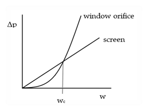
In Figure B-2, to the left of wc the laminar-flow screen pressure drop is higher, and to the right the orifice pressure drop dominates.
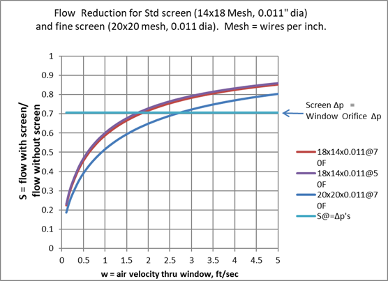
Figure B-3 shows S as a function of air velocity w for two common screen sizes. For the Standard screen, wc is 1.9-ft/sec. [At w = ~ 1-ft/sec taken as typical according to note #1, S = 0.6, corresponding to a 40% reduction in flow].
Figure B-3: Standard Screen Flow Reduction
Partial Derivatives for use in Airnet:
From Equation B-4 and Equation B-12,
Equation B-14

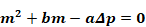
This can be written in the quadratic form for m:
Equation B-15
Where,


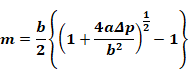
The single real root of the quadratic Equation B-15 gives the mass flow rate through a screen in series with a window-orifice as a function of screen and window properties and overall pressure drop:
If Δp is taken as Δp=P1-P2, then the partial derivative of m with respect to is P1
Equation B-17
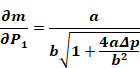
Equation B-18

These derivatives are needed in the Newton-Raphson procedure.
The derivatives Equation B-17 and Equation B-18 do not become unbounded
when Δp=0, as does the orifice Equation B-6, so that no special treatment
is needed near
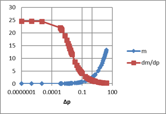
But the derivatives do become a little peculiar near zero
Δp as shown in Figure B-4 and Figure B-5. The value of a/b≈25, and
for thse plots for the standard screen of Figure B-3. It is possible this could cause problems in the N-R method, but testing AirNet with this type of element is the easiest way to find out.
Figure B-4: For Small Δp
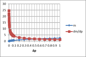
Figure B-5: For Large Δp