
There are four battery control strategies enabled in CBECC-Res as of May 2018: “Basic”, “Time of use” (TOU), “Advanced DR Control”, and “Advanced Control (old)”. These strategies are responsible for the timestep-by-timestep charge requests that are sent to the CSE battery module.
The Basic strategy charges when a) production exceeds demand and b) the battery is not fully charged and discharges when a) demand exceeds production and b) the battery is not fully drained. That is, the battery both charges and discharges as soon as it can.
charge_request = -load_seen
By charging from any excess production and discharging as soon as it can to serve load, the basic strategy maximizes self-consumption of the on-site PV production. The other strategies account for the time-varying value of electricity (e.g., as measured by TDV) to varying degrees to increase the TDV-savings the battery provides.
Figure 2: Illustrations of the battery control strategies’ different responses to a single day. Note that the TOU and Advanced strategies can discharge directly to the grid. Also notice that Advanced charges the battery from PV while serving loads from the grid.
The TOU strategy attempts to preferentially discharge during high-value hours during summer months (July-September). Charging rules are the same as the basic strategy. The discharge period is statically defined (per climate zone) by the first hour of the expected evening TDV peak. Consider a summer day in which the evening peak is defined to start at 20:00 but during which simulation load exceeds PV production during the 19:00 hour. While a simulation utilizing the Basic strategy would discharge to neutralize the net load during the 19:00 hour, a simulation on the TOU strategy would reserve the battery until 20:00 before commencing discharge. Because the TDV at 20:00 is likely to be higher than the TDV at 19:00, this strategy of reserving the battery for higher-value hours results in a lower (better) annual TDV.
A second difference: During the peak window, the battery is permitted to discharge at full power, even exceeding the site’s net load. This is in contrast to the Basic strategy, which is limited to the net load.
if this_hour
<
first_peak_hr:
charge_request = -min(load_seen, 0) // only
charge
else:
charge_request = -1000 // maximum discharge
Outside of July-September the TOU strategy reverts to the Basic strategy.
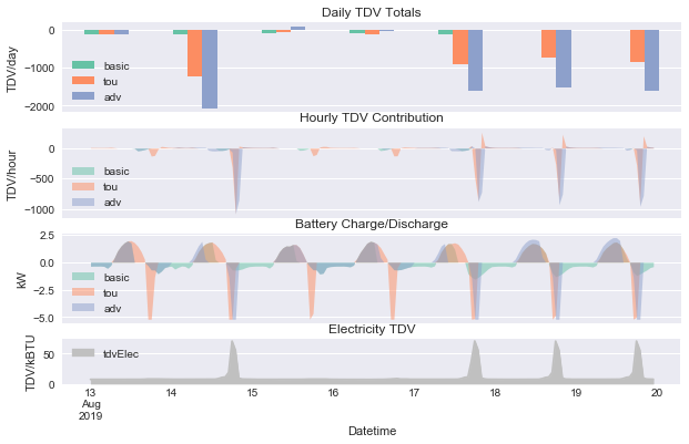
Figure 3: On days with high Electricity TDV, the TOU and Advanced control strategies can accumulate large negative TDV by discharging to the grid during peak hours. The Advanced strategy specifically targets the top three TDV hours each day for discharging
The Advanced DR (i.e., Demand Response) strategy uses the current day’s TDV schedule to make dynamic time-of-use priorities. This strategy activates on days that have a peak TDV greater than 10 TDV/kBTU. On all other days, the simulation reverts to the Basic strategy.
On a peak day (as defined by a peak greater than 10 TDV/kBTU), the strategy finds the top three hours by TDV. The algorithm asks for full discharge during the top two hours and uses the remainder during the third-highest hour. The ‘top three hours’ is hardcoded: the strategy assumes the battery holds between two and three hours of charge. If simulations are to allow other battery storage ratios, the algorithm will have to be upgraded.
As with the TOU strategy, the
battery may discharge in excess of net load during peak hours.
The
Advanced DR strategy is also allowed to charge from the PV system before production overtakes
load. Whereas the Basic and TOU strategies only charge with surplus production,
this strategy will—on a peak day—charge from the first PV production
available.
if day_tdv_peak > 10:
if tdv_rank(this_hour) in [1, 2]:
// maximum discharge top two TDV hours
charge_request = -1000
else if tdv_rank(this_hour) == 3:
// in third TDV hour, use remaining charge
charge_request = max_capacity -
2*(max_discharge_rate/η_discharge)
else:
// charge from PV, without subtracting load
charge_request = pv_production
else:
// on non-peak days, revert to basic strategy
charge_request = -load_seen
The “Advanced Control (old)” strategy is an omniscient system that runs two simulations to fine-tune the battery operation to minimize overall TDV. The first simulation--run without a battery--produces timeseries for load and PV production. An intermediate Python script compares the resulting net-load to a TDV timeseries and produces an optimal battery strategy for each day given that building-battery-array-weather-TDV combination. Unlike the other three strategies, which make charge/discharge decisions within the simulation, this strategy allows perfect foresight. The algorithmic details are described in a methodology report from Energy and Environmental Economics, Inc., the firm that wrote the Advanced Control (old) algorithm (E3, undated). This strategy is not available for compliance and is included in the program for research purposes only.
Battery Parameters Included in CBECC-Res/CSE
CBECC-Res allows the modeler to adjust a handful of battery parameters (Figure 4):
•Battery capacity (kWh): the CBECC-Res software enforces a 5kW minimum size for the battery to qualify for the Self Utilization Credit.
•Control strategy, chosen from the four options described in the Battery Control Strategies section of this paper.

Figure 4: The CBECC-Res battery dialog allows the modeler to set battery capacity, control strategy, and charge/discharge efficiencies. (Source: screenshot of CBECC-Res software user interface.)
•Charging and discharging efficiency (fraction): CSE allows charging and discharging efficiencies to be defined independently. The CBECC-Res default is 0.95 for each, resulting in a default round-trip efficiency of 0.9025.
•The CBECC-Res interface only requires that the efficiency inputs be between 0 and 1 (inclusive). A model operator could set both inputs to 1.0 and model a fictional lossless battery.
CBECC-Res also makes a set of assumptions to set CSE battery parameters. These are parameters that can be set in the lower-level CSE but that CBECC-Res defines itself.
•CBECC-Res assumes that the input battery capacity is the capacity of a brand new system. To account for aging across the battery’s life cycle (see the “Battery lifetime, aging, and degradation” section of this paper), the software derates the effective battery capacity to 85% of the input battery capacity. A nominal 10 kWh battery gets 8.5 kWh of usable capacity in the simulation.
•The 85%-of-input-capacity figure interrelates with the fact that battery systems often have different published values for total and usable capacity. The battery management system prevents complete discharges, so the usable capacity is typically single-digit percents lower than the total capacity (e.g., the Powerwall 2 has 14 kWh total and 13.5 kWh available energy). CBECC-Res should clarify whether the input capacity should be total or useful, and the degradation derate figure should be consistent with the input CBECC-Res expects.
•CBECC-Res derives the CSE parameters Maximum charge rate and Maximum discharge rate (kW/hr) from the battery capacity. They are each defined to be battery capacity * 0.42. That is, the battery is sized to have 2.38 hours of storage at full discharge. (1/0.42 = 2.38). That ratio is likely derived from the 14 kWh capacity and 5 kW discharge power of the Powerwall 2: 14 * 0.85 / 5 = 2.38.
•The battery is assumed start the simulation fully discharged. It is not required to be fully charged at the conclusion of the simulation.
•Battery-PV installations come in a range of electrical configurations, sometimes with independent inverters for each component (AC-coupled), sometimes sharing an inverter (DC-coupled). CSE assumes an AC-battery-module electrical configuration as shown in Figure 5. The modeling implication of that configuration is that the user-input battery charge and discharge efficiencies should include the losses associated with the battery module’s onboard inverter. In CSE, the PV system always has a dedicated PV inverter.

Figure 5: General layout diagram of an AC battery module layout of a residential PV-battery system. (Source https://www.cleanenergyreviews.info/blog/ac-coupling-vs-dc-coupling-solar-battery-storage.)
Simulated battery performance is static in the current CSE implementation. In particular, charge and discharge efficiencies do not vary with either charge rate or temperature. In real-world battery systems, efficiency falls from the benchmark a) with age, b) under rapid charging/discharging, and c) when temperatures are outside an ideal range (e.g., 25 °C/77 °F).
A real-world battery’s available capacity is also subject to age and external conditions. Low temperatures, especially, reduce a battery’s in-the-moment available capacity. CSE neglects those effects as well. The long-term dynamics of how batteries age warrants its own section, below.
The existence of a battery in the CBECC-Res model also relaxes size limits on PV systems. Without onsite storage, the PV system is limited by the interconnection rule: solar generation must not exceed the building’s electricity consumption over the course of a year. Title 24, Part 6 allows a building with a battery larger than 5 kWh to have a PV system that produces up to 1.6 times the building’s annual electricity consumption. The CBECC-Res software implements this change.