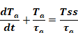
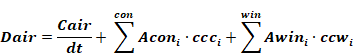
Similar to the energy balance on the construction mass nodes, an energy balance on the air node gives the differential equation:
Equation 8
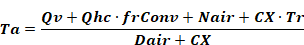
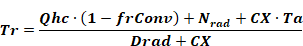
Where Tss, the asymptotic steady state temperature of Ta, includes all the sources connected to Ta. For simplicity, if the zone only contained the one construction (i = 1) and one window (j=1), like in Figure 3, then from a steady state energy balance Tss is given by:
Equation 9


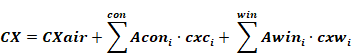
Where
Equation 10
CX=CXair+CXW1+CXC1
Equation 11

and the air time constant is:
Equation 12

Equation 8 is solved using an full implicit (or backward time) difference, similar to the Euler explicit method except here the right hand side of the equation remains constant over the time step at its value at the end of the time step, not its value at the beginning as in the Euler method. Thus, then becomes:
Equation 13
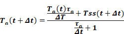
Where the times t and t+Δt in parenthesis indicate the terms are evaluated at the beginning and end of the time step, respectively. Substituting Equation 12 for τa, Equation 13 can be put in the convenient form:
Equation 14
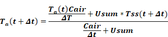
As this equation shows, with the implicit difference the effect of the air mass can be thought of as a resistance, Δt/Cair, between the Ta node and a fictitious node set at the air temperature at the value it was at the beginning of the time step, TaL = Ta(t). This alternative is known as an 'associated discrete circuit'. Leaving out the explicit time references, Equation 14 can be written:
Equation 15
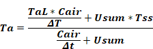
where Ta and Tss are evaluated at the end of the time step, and TaL stands for Ta(t) at the beginning of the time step. Note that Equation 15 still contains the variable Tr (hidden in Tss) which is unknown. Tr can be eliminated by making an energy balance on the Tr node and substituting the expression for Tr into Equation 15. This is done for the complete set of equations that follow.
The complete set of zone energy balance equations for multiple windows and constructions are given below. Terms containing Qv and Qhc are kept separate so that the resulting equations can be solved for Qv or Qhc when Ta is fixed at a setpoint.
The energy balance equation on the Ta node, comparable to Equation 15 above is:
Equation 16
The Equation 16 form, using Qv, is used when heat is transferred to a conditioned zone with ventilation or infiltration air. When heat is transferred to an unconditioned zone due to ventilation or infiltration, Qv is replaced by the essentially equivalent form given by Equation 17, wherein Qv is replaced by Qv=mCpΔT such that mdot*cp*T is added to the numerator and mdot*cp is added to the denominator. This was implemented to eliminate oscillations in Ta.
Equation 17
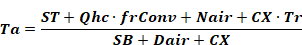
where,
Equation 18
ST=∑ mdot*cp*T
where T is the temperature of the air in the zone supplying the infiltration or ventilation air.
Equation 19
SB=∑ mdot*cp
Equation 20
with the sum's for all constructions and all windows respectively.
Equation 21
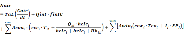
Equation 22
Qv is the heat transfer to the air node due to infiltration and forced or natural ventilation.
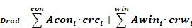
An energy balance on the Tr node gives Equation 23.
Equation 23
where,
Equation 24

Equation 25
Equation 16 and Equation 23 can be solved simultaneously to eliminate Tr and give Ta explicitly:
Equation 26

Similar to Equation 16 and Equation 17 the alternate form of Equation 26 is given by Equation 27
Equation 27

Substituting Equation 26 into Equation 23 gives
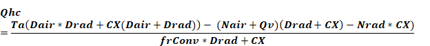
When Ta is at either the heating or cooling setpoints, Equation 26 is solved to determine the required Qhc. In this case Qv is set to QvInf.
Equation 28
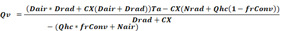
Similarly, when Ta is at the ventilation setpoint, Equation 26 can be solved for Qv to give:
Equation 29
With Qhc = 0 this becomes:
Equation 30

The zone balance is essentially an instantaneous balance, so all the temp inputs are simultaneous values from the end of the time step (with the exception of TaL; see Section 2.3.1). Although the balance is with contemporary temperatures, many of the heat flows in Nair etc., are based on last time step conditions.
At the end of each time step the program finds the floating temperature of the zone without HVAC (Qhc=0) and with venting . Qv=QvInf. This floating temperature found from Equation 26 is defined as TS1. Next, the venting capacity is determined (see Section 2.9.3.10, Heat Flow), and Equation 26 is solved for Ta at the full venting capacity. This Ta is defined as TS2.
TS1 will satisfy one of the four cases:
•TS1>TC
•TC > TS1 > TD
•TD > TS1 > TH
•TH > TS1
Similarly, TS2 will satisfy one of the four cases:
•TS2 > TC,
•TC > TS2 > TD
•TD > TS2 > TH
•TH > TS2
where TC, TD, and TH are the scheduled cooling, ventilation, and heating setpoints, with TC > TD > TH.
Based on the cases that TS1 and TS2 satisfy, nested logic statements determine the appropriate value of heating, cooling, venting, or floating .
For example, if TS1 and TS2 are both > TC, then Qv is set QvInf and Ta is set to TC, and Equation 28 is solved for the required cooling, Qhc. If Qhc is smaller than the cooling capacity at this time step then Qhc is taken as the current cooling rate and the zone balance is finished and the routine is exited. If Qhc is larger than the cooling capacity then Qhc is set to the cooling capacity, and Equation 26 is solved for Ta, floating above TC due to the limited cooling capacity. If Ta < TS2 then Ta and Qhc are correct and the zone balance routine is exited. If this Ta > TS2 then Ta is set equal to TS2, Qhc is set to zero, and Equation 29 is solved for the ventilation rate Qv, and the Zone Balance routine is complete.
Similar logic applies to all other logically possible combinations of the TS1 and TS2 cases above.
The limiting capacity of the heating and cooling system is determined each time step by multiplying the scheduled nominal air handler input energy capacity by the duct system efficiency. To avoid iteration between the conditioned zone and unconditioned zone simulations, the duct system efficiency is taken from the last time-step’s unconditioned zone simulation, or unity if the system mode (heating, cooling, venting, or floating) has changed.