The radiant model used in CSE is based on the “MRT Network Method” developed by Joe Carroll (see Carroll 1980 & 1981, and Carroll & Clinton 1980 & 1982). It was chosen because it doesn’t require standard engineering view factors to be calculated, and yet gives a relatively accurate radiant heat distribution for typical building enclosures (see Carroll 1981).
It is an approximate model that simplifies the “exact” network (see Appendix C) by using a mean radiant temperature node, Tr, that act as a clearinghouse for the radiation heat exchange between surfaces, much as does the single air temperature node for the simple convective heat transfer models. For n surfaces this reduces the number of circuit elements from (n-1)! in the exact case, to n with the Carroll model.
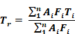
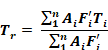
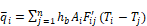
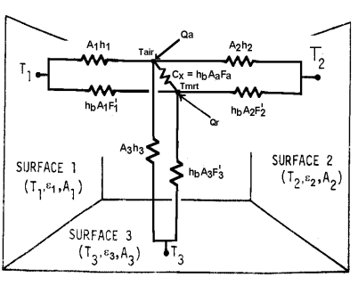
For black surfaces the radiant network is shown in Figure 8. For n surfaces, Tr floats at the conductance, , Ai Fi weighted average surface temperature:
Equation 77
The actual areas,
Figure 8: Carroll Network for Black Surfaces
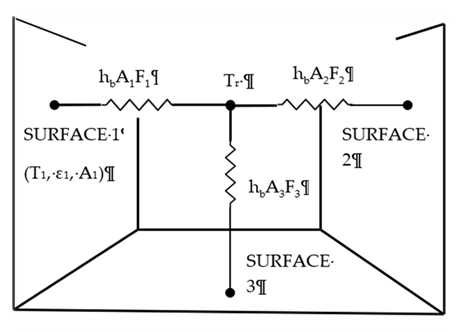
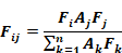
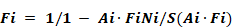
The factor Fi, in the radiant conductance
between the Ti surface node and the Tr node i
in the temperature Tr. The Fi factors are obtained from
the set of n nonlinear equations for n surfaces:
i
in the temperature Tr. The Fi factors are obtained from
the set of n nonlinear equations for n surfaces:
Equation 78
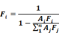
Given the surface areas, these equations are easily solved at the beginning of the simulation by successive substitution, starting with all Fi=1. This converges for realistic enclosures, but won’t necessarily converge for enclosures having only two or three surfaces, particularly if there are large area disparities.
Fi is always larger
than 1 because it’s role is to raise the conductance between Tr and
Ti to compensate for the potential
difference |Tr - Ti |being smaller than it would be
had Ti not been part of the conductance weighted average
 i values
can be seen to be close to 1, since
i values
can be seen to be close to 1, since
Equation 78 is roughly approximated by
The net radiant heat transfer [Btu/hr] from surface
Equation 79
Using a Y-Δ transformation, the
Figure 8 circuit can put in the form of the exact solution network of Figure
C-1 in Appendix C, showing the implicit view factors
Equation 80
Thus the implicit view factors are independent of the relative spacial disposition of the surfaces, and almost directly proportional to the surface area Aj of the viewed by surface i. Also, without special adjustments (see Carroll (1980a)), all surfaces see each other, so coplanar surfaces (a window and the wall it is in) radiate to each other.
Equation 79 is exact (i.e.,
gives same answers as the Appendix C model) for cubical rooms; for which
Equation 78 gives Fi=1.20. Substituting this into Equation 80 gives the implied Fij=0.2. This is the correct Fij for cubes using view-factor equations Howell(1982). It is likely accurate for all of the regular polyhedra.
Grey surfaces
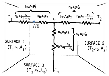
Carroll’s model handles gray surfaces, with emissivities,
εi by adding the Oppenheim surface conductance 
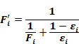
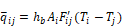
in series with the conductances hb Ai Fi . As shown in Figure 9, the conductance between Ti and Tr becomes hb Ai Fi where the Fi' terms are:
Equation 81
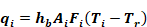
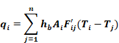
The net radiant heat transfer [Btu/hr] from surface i is given by
Equation 82
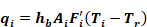
where for grey surfaces Tr is the " hb Ai Fi" weighted average surface temperature given by:
Equation 83
Similar to Equation 77 for a black enclosure, Equation 83 shows that Tr for grey surfaces is the conductance, Ai Fi, weighted average surface temperatures.
The role of Fi hasn’t changed, but since the
conductance Ai Fi is now connected to the radiosity node
rather than the surface node, i Fi-weighted average radiosity of the surfaces,
rather than the AiFi -weighted average emissive power of
the surfaces as in the black enclosure case.
i Fi-weighted average radiosity of the surfaces,
rather than the AiFi -weighted average emissive power of
the surfaces as in the black enclosure case.
Figure 9: Carroll Radiant Network for Grey Surfaces
This completes the description of the basic Carroll model. The principle inputs are the interior surface areas in the zone, the emissivities of these surfaces, and the typical volume to surface area ratio of the zone (see Section 2.6.1.3). All of the interior surfaces, including ducts, windows, and interior walls, are assumed to exchange heat between each other as diffusely radiating gray body surfaces.
Longwave radiant internal gains can be added, in Btu/hr, to
the radiant node Tr. This distributes the gains in proportion to the conductance
Conversion to delta
Using a Y-Δ transformation, the radiant network of Figure 9 can be converted to the Appendix C, Figure C-3 circuit form, eliciting the Fij' interchange factors implicit in Carroll’s algorithm. Similar in form to Equation 80,
Equation 84
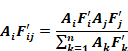
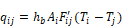
Using these
values, qij can be obtained from
Equation 85
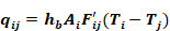
The total net heat transfer from surface i (i.e., the radiosity minus the irradiation for the un-linearized circuit) is given by summing Equation 85 for all the surfaces seen by surface i:
Equation 86
which will agree with the result of Equation 82.
The Carroll model of Figure 9 is exact for cubical enclosures with arbitrary surface emissivities. It is surprisingly accurate for a wide variety of shapes, such as hip roof attics and geodesic domes.
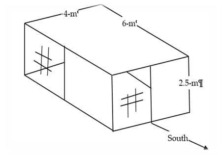
Carroll (1981) compared his model, and other simplified models, with the exact solution for the enclosure shown in Figure 10. Half the south wall and half of the west wall are glass with ε = 0.84, and the rest of the interior surfaces have ε = 0.9.
Figure 10: Test Room of Walton (1980)
Comparisons were made primarily regarding three types of errors:
Heat balance errors
The first law requires that the sum of the net radiation
emitted by each of the surfaces, plus any internal gain source of
long-wave radiation, must equal zero. That is,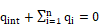
Due to their fixed conductance circuits, both the Carroll method and the Walton(1983) method are inherently free of heat balance errors. Carroll found BLAST and NBSLD algorithms to have rms heat balance errors of 9.8% (12%) and 1.7%(3.4%) for the Figure 10 enclosure.
Individual surface net heat transfer errors
For a given enclosure, these are errors in an individual
surfaces net heat flow, qi, compared to the exact method. For
Carroll’s method, this finds the error in qi, determined from the
values of
Equation 84, compared to the qi, values found using the exact
values (obtainable from Figure C-3 of Appendix C).
Carroll found the % rms error in the qi, values for a given enclosure in two different ways.
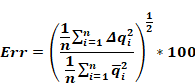
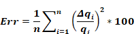
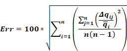
The first method, Equation 87, gives the rms error of qi, for each surface divided by the rms of the n net heat transfers from each surface:
Equation 87
where

is the error in

using Fij'values from Carroll’s model, Equation 87.
using the exact Fij values of Figure C-3 of Appendix C.

assumed in all cases.
n = the number of surfaces
The second method, Equation 88, gives the rms of the percentage error in qi f each surfaces. This method increases the weight of smaller surfaces such as windows.
Equation 88
Results
For the enclosure of Figure 10, Carroll found his method gives Err = 0.11% for the first method and 0.19% for the second method.
These results are shown in Table 4, along with the results for other shape enclosures, and the errors determined by Carroll using the radiant interchange algorithms of Walton (1980) and NBSLD and BLAST simplified models.
Table 4: Err = %rms Error in qi from Equation 87 and Equation 88 in Parenthesis
|
|
Figure 10 room 2.5:4:6 ε = 0.9 (.84 wdws) |
Corridor 10:1:1 ε = 0.9 |
10:10:1 ε = 0.9 |
|
Carroll |
0.11 (0.19) |
0.06(0.05) |
0.07 (0.04) |
|
Walton(1980) |
1.9 (1.30) |
0.6 (0.6) |
4.4 (3.0) |
|
NBSLD, BLAST |
3.2 (2.1) |
3.2 (2.6) |
7.5 (4.4) |
Errors in an individual surface’s distribution of heat transfer to other surfaces
These are errors in qij, the heat exchanged between surfaces i and j (both directly and by reflections from other surfaces), relative to the exact total net heat transfer from surface i given by Figure C-3 of Appendix C.
Carroll gives two percentage error results.
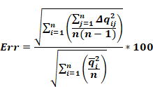
By the first method, for each surface i, the rms of the error, Δqij, in heat exchange to each of the n-1 other j surfaces is obtained. Then the rms of these n rms error values is obtained, giving a representative distribution error for the enclosure. Dividing this by the rms value of the exact net surface heat transfers, qi, of all the surfaces gives the final distribution error in percent:
Equation 89
where

With 
with the exact Fij' values of Figure C-3 of Appendix C.
By the second method, for each surface i, the rms of the percentage error in heat exchange qij relative to the exact net heat transfer from that surface, q ̅i,is obtained.
Equation 90
Distribution error results
For the Figure 10 room, Carroll’s model gives errors of 2.1% and 3.9% for methods 1 and 2 respectively. Walton’s model has corresponding errors of 2.4% and 3.7%. Equation 91 was used for the results in parenthesis.
Table 5: % rms Error in
|
|
Figure 10 room 2.5:4:6 ε = 0.9 (.84 wdws) |
Corridor 1:10:1 ε = 0.9 |
Warehouse 1:10:10 ε = 0.9 |
|
Carroll |
2.1 (3.9) |
3.3 (2.8) |
0.6 (1.9) |
|
Walton(1980 ) |
2.4 (3.7) |
3.3 (2.8) |
2.8 (3.0) |
|
BLAST |
2.8 (4.4) |
3.4 (4.4) |
3.4 (15) |
|
NBSLD |
1.7 (3.5) |
1 (0.83) |
3.3(1.9) |
(Equation 91 was used for the results in parenthesis.)
Carroll’s model is seen to give very respectable results, despite giving no special treatment to coplanar surfaces.
The Carroll model also accounts for the absorption of long-wave radiation in the air, so that the air and mrt nodes are thermally coupled to each other as well as to the interior surfaces. Carroll (1980a) gives an air emissivity by the following dimensional empirical equation that is based on Hottel data from McAdams(1954):
Equation 91
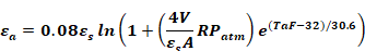
The logarithm is natural, and,
εs= the area-weighted average long-wave emissivity for room surfaces, excluding air.
V/A = the room volume to surface area ratio, in meters.
R = the relative humidity in the zone. (0 ≤ R ≤ 1).
Patm = atmospheric pressure in atmospheres.
Τa = zone air temperature, in °F.
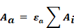
Following a heuristic argument Carroll assigns an effective
area Aa to the air
that is the product of εa and the sum of all of the
zone surface areas, as if the absorbing part of the air were consolidated into a
surface of area
Equation 92
Using this area, the value of Fa for this 'surface' can be calculated along with the other Fi by Equation 80. The value of the conductance between the air and radiant nodes in Figure 11 is given by:
Equation 93

Figure 11: Like Figure 9 but with Convective Network Added
Suppose one of the interior surfaces of total area Ai is composed of Ni identical flat sub-surfaces, each at the same temperature, and similar views to each other, like the facets of a geodesic dome. The Fi values would be the same if each facet is treated as a separate surface. To avoid redundant solutions to Equation 80, it is easy to show that Ai can be treated as one surface in Equation 6-4 if iNi is introduced into Equation 80 as follows:
Equation 94
The facet feature is utilized in the simulation to represent attic truss surfaces.
Short Wave Radiation Distribution
This routine was used in the development code for this program. It is not currently implemented in CSE, being replaced by a simplified but similar routine.
The short wave radiation (solar insolation from hourly input) transmitted by each window can, at the users discretion, be all distributed diffusely inside the zone, or some of the insolation from each window can be specifically targeted to be incident on any number of surfaces, with the remaining untargeted radiation, if any, from that window, distributed diffusely. The insolation incident on any surface can be absorbed, reflected, and/or transmitted, depending on the surface properties inputted for that surface. The radiation that is reflected from the surfaces is distributed diffusely, to be reflected and absorbed by other surfaces ad infinitum.
Since some of the inside surfaces will be the inside surface of exterior windows, then some of the solar radiation admitted to the building will be either lost out the windows or absorbed or reflected by the widows.
Assume a spherical zone with total insolation S(Btu/hr)
admitted into the zone through one window. Assume that the portion 2*Btu/(hr-ft2))
Of S (Btu/hr) is targeted to surface i with area ai such that,
Equation 95

where the sum is over all surfaces i. The total
spherical area is
Also incident on surface i will be the irradiation Gi (Btu/hr-ft2) from other surfaces that have reflected a portion of the radiation they have received. We distinguish between the Qi incident on the surface directly from the window, and the irradiation Gi which is composed of radiation reflected to i from all the surfaces, and that reflected by windows. All radiation (including Incident beam) is assumed to be reflected diffusely.
Each surface i will also reflect short-wave radiation, with a radiosity Ji [Btu/hr-sf].
Figure 12: Radiation Terminology
Ji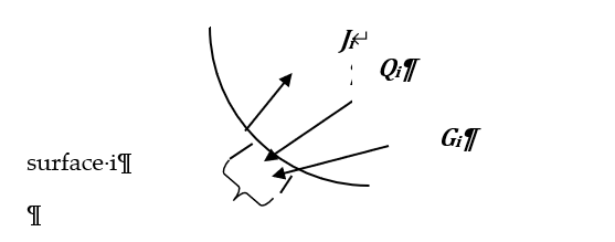

The derivation below determines the equations to obtain Ji and Gi for known Qi values, for all the surfaces of the sphere, i = 1 to n.
First a relationship between Gi and Ji is developed:
Since Gi is composed only of reflected radiation,
Equation 96
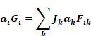
where the sum is over all surfaces n of the sphere of area aS.
Using the view-factor reciprocity principle,
Gi becomes
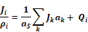
For spherical geometry, the view factor is Fik=ak/aS, where , aS=∑ak so Gi can be written
Equation 97
The right hand side is the area-weighted average radiosity, showing that Gi is independent of i,
Equation 98

Next a separate relationship between Ji and Gi is obtained, Gi eliminated and Ji solved for explicitly:
The radiosity of surface i is composed of the reflected part of both the irradiation and the targeted solar
Equation 99
Substituting Equation 97 for Gi gives
Equation 100
Since by Equation 98 Gi is independent of i, then Equation 99 shows that the radiosity of any surface i is related to the radiosity of any surface k by the relationship
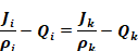
Substituting this into Equation 100 gives
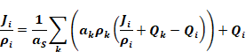
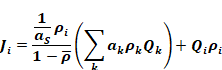
This can be solved explicitly for 
Equation 101
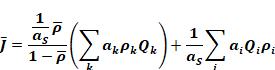
From Equation 101, the area weighted average J is
Equation 102
where
is the area weighed average reflectivity.
Now that  and
and  are known an
energy balance will give the net heat transfer:
are known an
energy balance will give the net heat transfer:
The net energy rate (Btu/hr) absorbed and/or transmitted by surface i, is:
Equation 103

Substituting Equation 101 and Equation 102 into this gives
Equation 104
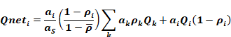
The first term in Equation 104 is from the absorption and/or transmission of radiation that reached and is absorbed by surface i after having been reflected, ad infinitum, by the interior surfaces. The second term is from the absorption of the "initially" incident insolation Qi on surface i.
If none of the insolation is specifically targeted, and instead S is assumed to be distributed isotropically then Qi is the same for each surface:
Equation 105

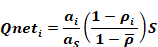
Substituting this into Equation 104 gives Qneti for isotropically distributed insolation:
Equation 106
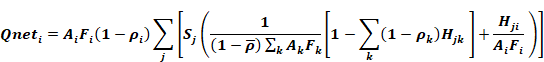
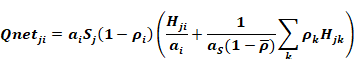
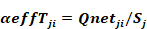
The targeting can be different for each window. Adding an additional subscript
"j" to Equation 104 allows it to represent the energy removal for each surface
separately for each window j. That is, Equation 104 becomes Equation 107, the
rate of energy removal at each surface due to insolation Sj,
that is distributed according to the assigned targeted values 
Equation 107

The targeting fractions Hjk to be user input, are defined as the fraction of insolation from window j that is incident on surface k:
Equation 108

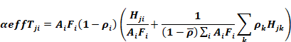
With this definition, Equation 107 can be written as
Equation 109
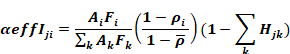
The effective absorptivity of the targeted surfaces is defined as
Equation 110
Replacing the spherical surfaces ai in Equation 107 by ai=Ai Fi, and substituting Equation 109 into Equation 110 gives the targeted gain equation used in the CZM code:
Equation 111
If ∑kHjk<1 then it is assumed that the remaining insolation Sj(1-∑kHjk) is distributed isotropically. From Equation 105 it is
Equation 112
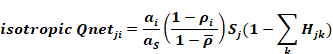
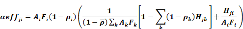
The definition of the effective absorptivity for isotropic insolation is:
Equation 113
Changing Equation 112 to utilize zone areas, ai=Ai Fi and substituting Equation 112 into Equation 113 gives the amount of the diffuse part of the insolation from each window j that is
Equation 114
Note that no distinction has been made between surfaces that are opaque like walls, and partially transparent window surfaces. They are treated equally. The difference is that the energy removed by an opaque wall is absorbed into the wall, whereas that removed by the window surfaces is partly transmitted back out the window, and partly absorbed at the window inside surface. The CZM development code lets the user specify a fraction of the radiation that is absorbed in the room-side surface of the window, which slightly heats the window and thus the zone.
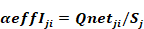
Adding Equation 111 and Equation 114 gives the total effective absorptivity of surface i from the insolation admitted through window j:
Equation 115
The net radiation absorbed in surface i from window j is thus
Equation 116
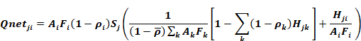
Summing this over all windows gives the total SW radiation absorbed and/or transmitted by surface i as:
Equation 117